This repo would contain important data science and ML interview questions.
What proportion of positive identifications was actually correct?
Mathematically, it is defined as follows:
Precision: TP/(TP+FP)
What proportion of actual positives was correctly identified?
Mathematically, it is defined as follows:
Recall: TP/(TP+FN)
Consider following example:
Suppose our model is tasked with analysing and classifying 100 scans of tumours as malignant(positive class) and benign(negative class). Let's say, the model is doing as following on the data:
- True Positive - Predicted: Malignant & Actual: Malignant -> 1
- False Positive - Predicted: Malignant & Actual: Benign -> 1
- False Negative - Predicted: Benign & Actual: Malignant -> 8
- True Negative - Predicted: Benign & Actual: Benign -> 90
So the model's accuracy comes out to be:
(TP+TN)/(TP+TN+FP+FN) = (1+90)/(1+90+1+8) = 0.91, i.e. 91%, pretty cool, right?
Let's dive deeper inside the results to gain more insight into our model's performance:
Of 100 tumour examples, 91 are benign (i.e. 90 TNs and 1 FP) and 9 are malignant (i.e. 8 FNs and 1 TP). Out of 91 benign tumours, the model classifies 90 images as benign correctly which is good, but out of 9 malignant tumours, it correctly identifies 1 image as malignant which is quite bad, as 8 out of 9 malignants got undiagnosed ! Another benign tumour classifier model which always predicts benign would achieve same level of accuracy for our dataset, means our model is no better than one that has zero predictive capacity to differentiate between malignant and benign tumours. So accuracy in this kind of cases would not capture the complete truth of the model's performance, where the dataset is class-imbalanced.
Let's calculate the precision and recall of the model:
Precision is TP/(TP+FP) = 1/(1+1) = 0.5. i.e. 50% means when our model predicts a tumour as malignant, it's correct 50% of the times
and
Recall is TP/(TP+FN) = 1/(1+8) = 0.11, i.e. 11% means our model correctly identifies 11% of all malignant tumours.
To better explain the answer to this question we have to understand the notion of false positive and false negative, i.e. Type I and Type II error respectively. False positive or Type I error occurs when the null hypothesis is rejected but in fact it was true. And we commit Type II error when the null hypothesis is accepted but in fact it was false.
Suppose, we have developed a model to determine a stock will be good for investment or not. Here the +ve class is 'good for investment' and -ve class is 'not good for investment'. We are not concerned with mislabelling a good stock as not good, i.e. False negative is not so important in this use case because we can afford to miss few profitable stock here and there as long as our money is going to an appreciating stock correctly predicted by our model. Rather if we mislabel a bad stock as good that would be terrible. And we would want to reduce that, i.e. False positive. So Precision will be our go-to metric for evaluating our model's performance.
Let's say we have developed a poisonous apple classifier, i.e. The +ve class is poison and -ve class is not poison. We are not too concerned with mislabelling an apple as poisonous because we would rather be safe than sorry, i.e. False positive is not important for this use case. Rather if we miss poisonous apple and mislabel it as not poisonous, i.e.the False negatives get increased, the model will not be effectively perform. So Recall would be appropriate.
So, it entirely depends on the goal of your model to determine the appropriate evaluation metric for our model
ROC, i.e. Receiver Operating Characteristic curve is a graph of true positive rate vs false positive rate at different classification thresholds, showing the performance of a classification model in binary classification. And AUC, i.e. Area Under the ROC Curve, represents the entire two-dimensional area underneath the entire ROC curve and ranges between 0.0 and 1.0
The shape of a ROC curve suggests a binary classification model's ability to separate positive classes from negative classes. For example, the following illustration shows a binary classification model perfectly separates all the negative classes from all the positive classes:
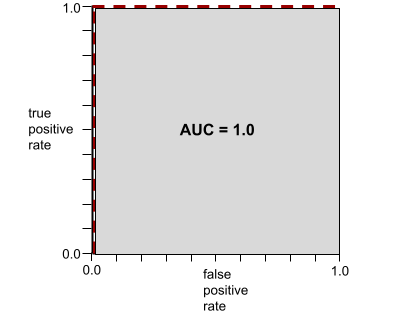
The ROC curve and the AUC (which is 1.0, the max possible value of AUC) for this unrealistically perfect model are shown in the following illustration:
On the other hand, the following illustration shows the raw and random values of a terrible model that can't separate negative classes from the positive classes at all:
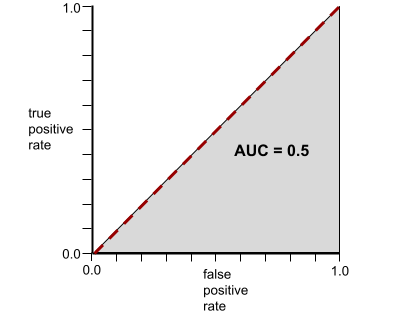
The ROC curve and the AUC (which is 0.5) for this model are shown in the following illustration:
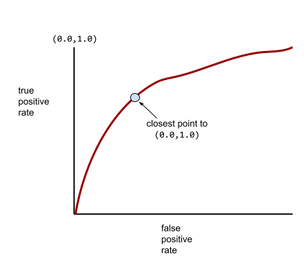
In the real world, most binary classification models separate positive and negative classes to some degree, but usually not perfectly. So, a typical ROC curve falls somewhere between the two extremes:
The point on an ROC curve closest to (0.0,1.0) theoretically identifies the ideal classification threshold. However, several other real-world issues influence the selection of the ideal classification threshold. For example, perhaps false negatives cause far more pain than false positives.
AUC ignores any value you set for classification threshold. Instead, it considers all possible classification thresholds. It summarizes the ROC curve into a single floating-point value and provides an aggregate measure of performance across all possible classification thresholds.
One way of interpreting AUC is as the probability that the model ranks a random positive example more highly than a random negative example, i.e. classifier will be more confident that a randomly chosen positive example is actually positive than that a randomly chosen negative example is positive.
The classification threshold is set by human and changing value of it directly influences the counts of false positives and false negatives which in turn impacts the true positive rate and false positive rate. The ROC curve therefore plots different sets of TPR & FPR for different classification thresholds for a binary classification problem. So it is unrealistic to think about plotting a single TPR and FPR in ROC curve which plots TPR and FPR for all possible classification thresholds.
As the backpropagation algorithm advances backward (or downwards) from the output layer towards the input layer, the gradients, in some cases, keep on getting larger and larger which in turn, causes very large weight updates and causes the gradient descent to diverge. Exploding gradient is the tendency for gradients in deep neural network to become surprisingly steep (high). Steep gradients often cause very large updates to the weights of each node in a deep neural network.
On the contrary, in some cases, the gradients keep on getting smaller and smaller and approach zero which eventually leaves the weights of the initial or lower layers nearly unchanged. As a result, the gradient descent never converges to the optimum. Vanishing gradient is the tendency for the gradients of early hidden layers of some deep neural networks to become surprisingly flat (low). Increasingly lower gradients result in increasingly smaller changes to the weights on nodes in a deep neural network, leading to little or no learning.
Models suffering from both the problems become difficult or impossible to train.
Selecting proper network architecture
Proper weight initialisations
Selection of proper activation function
Batch Normalisation
Proper optimiser with a well-tuned learning rate
*** Specific to Exploding Gradient Problem:***
Gradient Clipping
It is one of the most effective ways to mitigate exploding gradient issue by capping all the components of gradient vectors, i.e. the partial derivatives to a predetermined gradient threshold during backpropagation so that they never exceed the threshold. It is specially used in RNN.
The threshold value is a hyperparameter. The clipping operation for the gradient vectors can be performed in various ways. One of the most common ways is to rescale them in such a way that the norm of the error gradient vector is at most the threshold. This ensures that no gradient has a norm greater than the threshold
L2 norm regularisations
Specific to Vanishing Gradient Problem:
Reducing model complexity


