- 👨🏻💻 Author: Anderson H Uyekita
- 📚 Specialization: Data Science: Statistics and Machine Learning Specialization
- 📖 Course:
Regression Models
- 🧑🏫 Instructor: Brian Caffo
- 📆 Week 4
- 🚦 Start: Tuesday, 05 July 2022
- 🏁 Finish: Saturday, 09 July 2022
- 🌎 Rpubs: Interactive Document
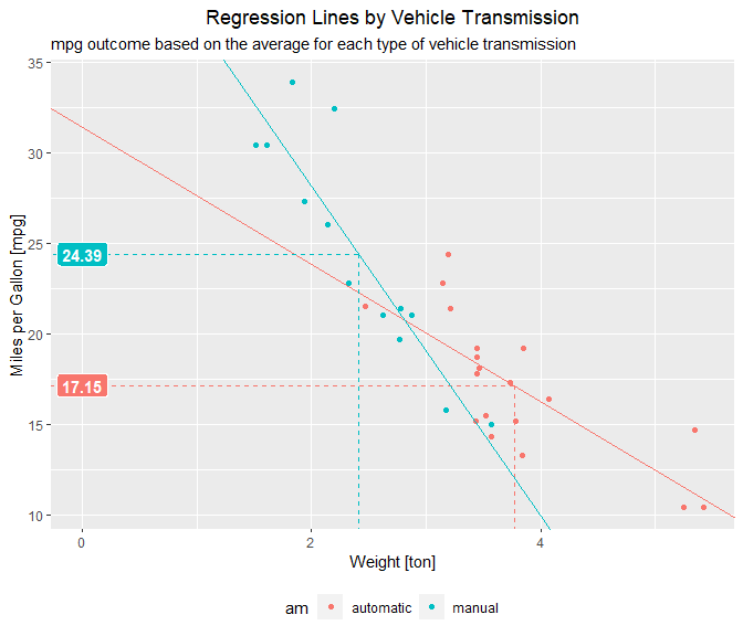
The data analysis process in this document has identified that manual
vehicles have better performance than automatics concerning miles per
gallon (mpg). Furthermore, based on this study’s linear regression
model, the difference has reached 7.24 miles per gallon based on the
average weights of automatic and manual cars (See Figure 4 in APPENDIX
Section A4.), which is a significant number.
The Motor Trend Car Road Test has evaluated 32 automobiles varying from 1973-74 models, and this study comprises fuel consumption, horsepower, weight, and other aspects. Based on it, the present publication aims to answer two questions:
- “Is an automatic or manual transmission better for MPG?”
- “Quantify the MPG difference between automatic and manual transmissions.”
If you are interested in reproducing this study, please visit the Github repository to have access to the raw document.
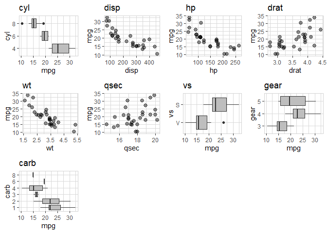
The adjusted data frame has 32 observations with no NA values, divided
into 6 (six) numeric variables (no one is standardized or scaled) and 5
(five) categorical variables. For more exploratory details, please, find
them in APPENDIX section A1. For more information about the variables
descriptions, please, see it on the R Documentation
website.
Due to Figure 2 in section A2 from APPENDIX, I have tested the
hypothesis that the average consumption from automatic and manual
vehicles is equal. In other words,
,
the p-value is 0.14% which is way less than alpha (5%). For this reason,
the
was Rejected, which means the averages of automatic and manual
transmissions are from different populations.
The model selection approach used for this project is based on the Week 3 videos and the Chapter Multiple variables and model selection from Regression Models for Data Science in R book.
The baseline model is the Ordinary Linear Regression, and this model
uses only transmission (am) to explain the consumption in miles per
gallon (mpg). From the hypothesis tested in Section 3, this baseline
model has identified that manual transmission performs better than
automatic ones. On average, manual transmission yields 24.39 miles per
gallon. On the other hand, automatic transmission yield 17.15 miles per
gallon. The difference is 7.24 miles per gallon.
Using the anova() function, it was possible to run several
combinations, reaching the final model using am, wt, and interaction
between am and wt.
I have decided to use a simpler model due to the parsimony. The R2 adjusted has reached 81.51%. All p-values of the model are below alpha (5%).
The linear model coefficients:
| Estimate | Std. Error | t value | Pr(\>\|t\|) | |
|---|---|---|---|---|
| (Intercept) | 31.416055 | 3.0201093 | 10.402291 | 0.0000000 |
| ammanual | 14.878422 | 4.2640422 | 3.489276 | 0.0016210 |
| wt | -3.785907 | 0.7856478 | -4.818836 | 0.0000455 |
| ammanual:wt | -5.298361 | 1.4446993 | -3.667449 | 0.0010171 |
Due to the low number of observations, below 50, I have used the Shapiro-Wilk test to ensure the residual’s normality. The p-value obtained from this test was 8.72%, sufficient to reject the null hypothesis and proving the residual’s normality.
The residual analysis will be based on Figure 3 in APPENDIX Section A3.. This figure aims to corroborate the following explanations:
- Residual vs. Fitted: The residual bounces around zero, which suggests an excellent linear relationship. Also, the residual is a homogeneous spread on the plot showing that the variance is “constant” in addition, I have identified no outlier.
- Normal Q-Q: Most of the data is around the line, except in the top right of the chart. I did not identify any issue related to non-normality.
- Scale-Location: There are no patterns in the points, the data stay between a fixed band, and the red line is almost constant. From those characteristics, the residual is considered homoscedasticity.
- Residual vs. Leverage: No points above the dotted line means there is no influential high point.
Considering the baseline model, the am variable can explain 33.85% of
the miles per gallon. However, In the final model, the percentage of
variance explained by the model rises to 81.51% with the inclusion of
two more predictors (wt and interaction of wt and am).
- Final model:
Figure 1 – Exploratory Data Visualization
Figure 2 – Fuel Consumption divided into Transmission and number of Gears.
Figure 3 – Residuals.
Figure 4 – On average, a manual car yields 7.24 more miles per gallon than automatics.


