This project is about taking cypto currency taken from Crypocurrency Data saved as csv and then using that to display the data using Table, Graph, and Candlestick. But that isnt the only thing that's happening, the data is also used for simple predictions that is Linear regression & Time series where their results will also be shown by a graph.
This project uses python and you can use any program like what i use, Pycharm to run the code. Before being able to run the code you will need to install these libraries:
- dash
- sklearn
- pandas
- plotly
- numpy
- keras
Dont forget to put the csv files in the same place as your code
Once you got your setup just run the code and it should be running on your localhost, in pycharm it will give you a link that you can click in the debbugger.
You can pick any of the given options of crypto currencies and everything will update

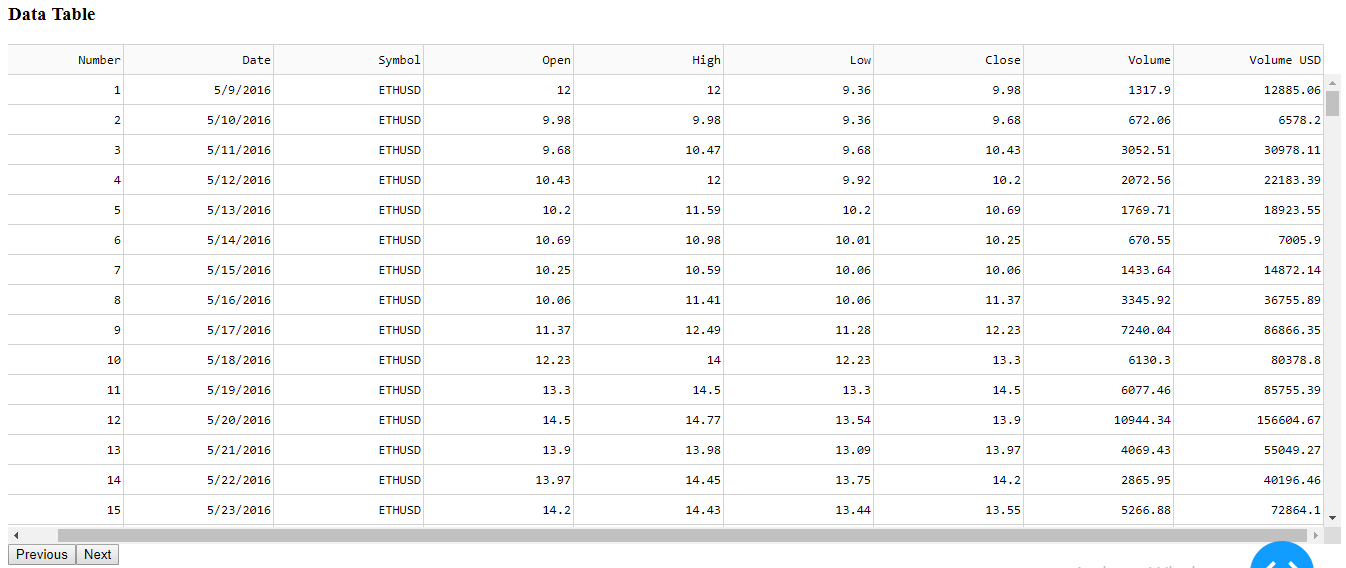
A table will show you all of the data contained in the csv provided. You will be able to go through every single column and row with the table.
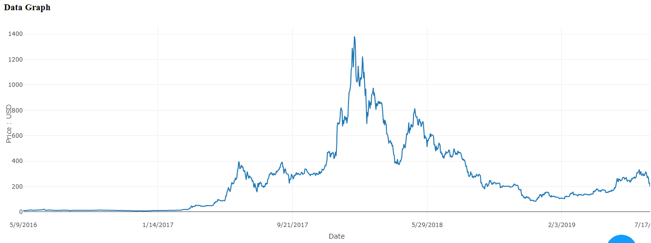
This graph will show you a line graph of the actual data.
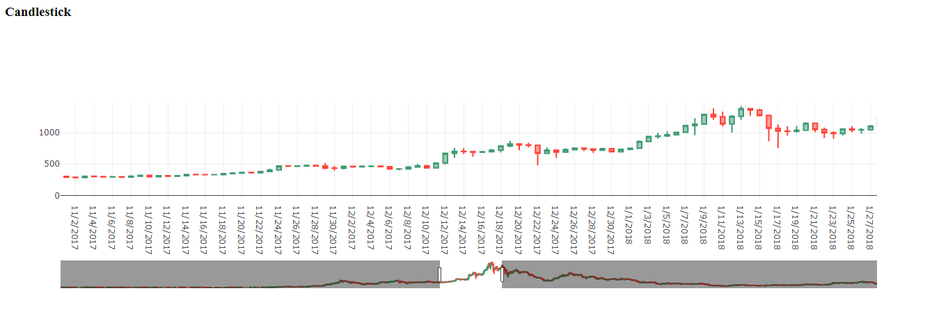
Since this is crypto currency so showing it with a candlestick would be optimal to show the complete actual data.
This is the most simplest and probably every data researcher first method in data science
@app.callback(Output('graph', 'figure'), [Input('table-dropdown', 'value')])
def update_graph(value_dropdown):
    if value_dropdown == 'BTC':
        df_to_graph = df
        df_graph = df
        text = 'Bitcoin'
        X = df.iloc[:, 0].values.reshape(-1, 1)  # values converts it into a numpy array
        Y = df.iloc[:, 4].values.reshape(-1, 1)  # -1 means that calculate the dimension of rows, but have 1 column
    elif value_dropdown == 'ETH':
        df_to_graph = dft
        df_graph = dft
        text = 'Ethirium'
        X = dft.iloc[:, 0].values.reshape(-1, 1)  # values converts it into a numpy array
        Y = dft.iloc[:, 4].values.reshape(-1, 1)  # -1 means that calculate the dimension of rows, but have 1 column

    linear_regressor = LinearRegression()  # create object for the class
    linear_regressor.fit(X, Y)  # perform linear regression
    Y_pred = linear_regressor.predict(X)  # make predictions

    df_for_graph = pd.DataFrame(Y_pred, columns=['Prediction'])

    return {
        'data': [go.Scatter(
            name='Linear Regression Prediction',
            mode='lines',
            x=df_to_graph['Date'],
            y=df_for_graph['Prediction'],
            text='Linear Regression Line',
            marker={
                'size': 15,
                'opacity': 0.5,
                'line': {'width': 0.5, 'color': 'blue'}
            }
        ),
            go.Scatter(
                name='Actual Data',
                mode='lines',
                x=df_graph['Date'],
                y=df_graph['Open'],
                text=text,
                marker={
                    'size': 15,
                    'opacity': 0.5,
                    'line': {'width': 0.5, 'color': 'red'}
                })
        ],
        'layout': go.Layout(
            xaxis={
                'title': 'Date',
                'tickvals': [df_to_graph['Date'].iloc[0], df_to_graph["Date"].iloc[250], df_to_graph["Date"].iloc[500],
                             df_to_graph["Date"].iloc[750], df_to_graph["Date"].iloc[1000], df_to_graph["Date"].iloc[-1]
                             ],
            },
            yaxis={
                'title': 'Price : USD',
            },
            margin={'l': 40, 'b': 40, 't': 10, 'r': 0},
            hovermode='closest'
        )
    }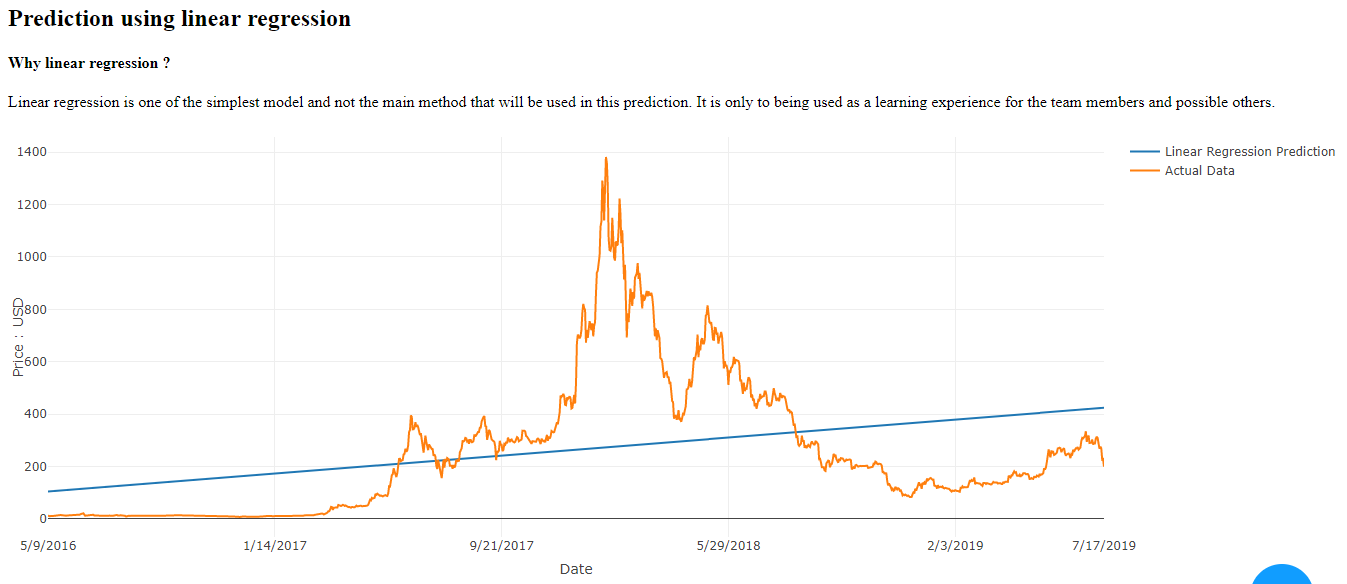
See screenshot after code to see what it produce
@app.callback(Output('graph-learn', 'figure'), [Input('table-dropdown', 'value')])
def update_graph_learn(value_dropdown):
if value_dropdown == 'BTC':
csv_name = 'Gemini_BTCUSD_daily.csv'
df_to_learn = df
elif value_dropdown == 'ETH':
csv_name = 'Gemini_ETHUSD_daily.csv'
df_to_learn = dft
# fix random seed for reproducibility
numpy.random.seed(7)
# load the dataset
dataframe = pd.read_csv(csv_name, usecols=[6], engine='python')
dataset = dataframe.values
dataset = dataset.astype('float32')
# split into train and test sets
train_size = int(len(dataset) * 0.67)
test_size = len(dataset) - train_size
train, test = dataset[0:train_size, :], dataset[train_size:len(dataset), :]
# reshape dataset
look_back = 3
trainX, trainY = create_dataset(train, look_back)
testX, testY = create_dataset(test, look_back)
# create and fit Multilayer Perceptron model
model = Sequential()
model.add(Dense(12, input_dim=look_back, activation='relu'))
# model.add(Dense(8, activation='relu'))
# model.add(Dense(1))
model.compile(loss='mean_squared_error', optimizer='adam')
model.fit(trainX, trainY, epochs=60, batch_size=2, verbose=2)
# Estimate model performance
trainScore = model.evaluate(trainX, trainY, verbose=0)
print('Train Score: %.2f MSE (%.2f RMSE)' % (trainScore, math.sqrt(trainScore)))
testScore = model.evaluate(testX, testY, verbose=0)
print('Test Score: %.2f MSE (%.2f RMSE)' % (testScore, math.sqrt(testScore)))
# generate predictions for training
trainPredict = model.predict(trainX)
testPredict = model.predict(testX)
# shift train predictions for plotting
trainPredictPlot = numpy.empty_like(dataset)
trainPredictPlot[:, :] = numpy.nan
trainPredictPlot[look_back:len(trainPredict) + look_back, :] = trainPredict
# shift test predictions for plotting
testPredictPlot = numpy.empty_like(dataset)
testPredictPlot[:, :] = numpy.nan
testPredictPlot[len(trainPredict) + (look_back * 2) + 1:len(dataset) - 1, :] = testPredict
dataset = pd.DataFrame(dataset, columns=['Data'])
trainPredictPlot = pd.DataFrame(trainPredictPlot, columns=['Train'])
testPredictPlot = pd.DataFrame(testPredictPlot, columns=['Test'])
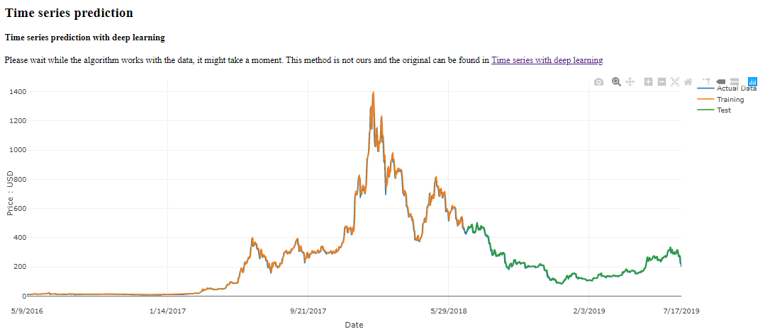
return {
'data': [go.Scatter(
name='Actual Data',
mode='lines',
x=df_to_learn['Date'],
y=dataset['Data'],
text='Actual Data',
marker={
'size': 15,
'opacity': 0.5,
'line': {'width': 0.5, 'color': 'blue'}
}
),
go.Scatter(
name='Training',
mode='lines',
x=df_to_learn['Date'],
y=trainPredictPlot['Train'],
text='Training',
marker={
'size': 15,
'opacity': 0.5,
'line': {'width': 0.5, 'color': 'green'}
}),
go.Scatter(
name='Test',
mode='lines',
x=df_to_learn['Date'],
y=testPredictPlot['Test'],
text='Test',
marker={
'size': 15,
'opacity': 0.5,
'line': {'width': 0.5, 'color': 'red'}
})
],
'layout': go.Layout(
xaxis={
'title': 'Date',
'tickvals': [df_to_learn['Date'].iloc[0], df_to_learn["Date"].iloc[250], df_to_learn["Date"].iloc[500],
df_to_learn["Date"].iloc[750], df_to_learn["Date"].iloc[1000], df_to_learn["Date"].iloc[-1]
],
},
yaxis={
'title': 'Price : USD',
},
margin={'l': 40, 'b': 40, 't': 10, 'r': 0},
hovermode='closest'
)
}
- Andreas Geraldo
- Thompson Darmawan Yanelie
- Jerry Aivanca Pattikawa
Crypto currency data - cryptodatadownload
Linear regression - towardsdatascience
Time series code - machinelearningmastery