txtools

Description

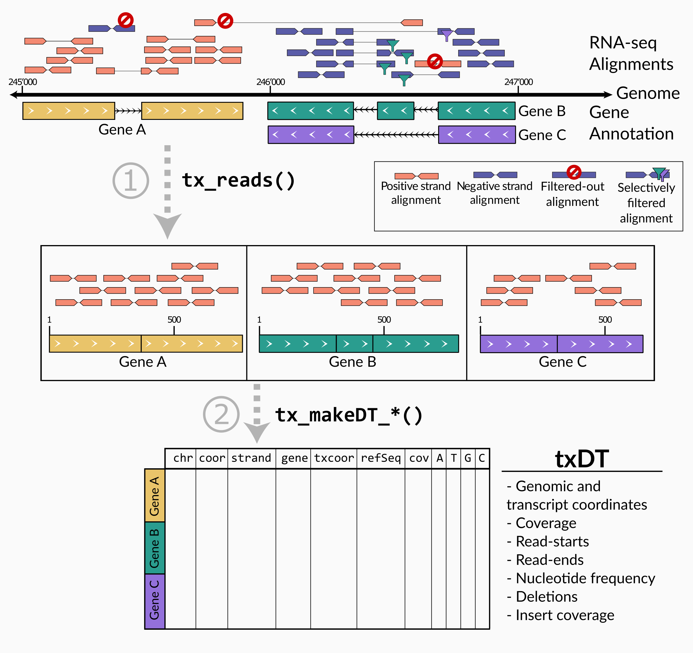
txtools is a package that processes RNA-seq reads alignments into transcriptomic-oriented tables. Enabling a quick and simplified analysis, to closely inspect summarized RNA-seq data per transcript, at nucleotide resolution, i.e. coverage, read-starts, read-ends, deletions, and nucleotide frequency. Attractive plotting is also readily available to visualize data.

The main processing pipeline of txtools consists of 1) converting genomic alignments into transcriptomic space and merging paired-end reads using tx_reads() and 2) summarize counts for ‘readouts’ (coverage, read-start, read-ends, nucleotide frequency, deletions) along the transcriptome using a function of the tx_makeDT_ family.

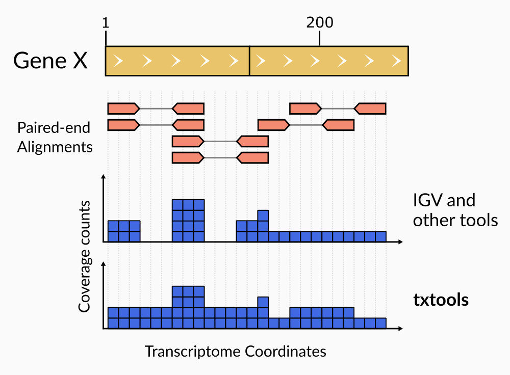
Figure 1. txtools’ main processing pipeline

Of note, coverage calculation in paired-end reads using txtools considers the whole range of the paired alignment. From the start of read1 to the end of read2, including the insert which is not directly sequenced (Figure 2)

Figure 2. Paired-end reads coverage computation

Installation

You can install the development version from GitHub typing in the following commands in the R console:

if (!requireNamespace("remotes", quietly = TRUE))
    install.packages("remotes")
remotes::install_github("AngelCampos/txtools", build_vignettes = TRUE)

Quick example

In this small example we use the ‘Pasilla’ experiment data (from its own package) which contains a BAM file for the paired-end alignments of a D. melanogaster RNA-seq experiment on chromosome 4, along with a FASTA file comprising the genome sequence for the same chromosome.

Using txtools we can load the genome (FASTA), the gene annotation (BED-12), and the RNA-seq reads alignment (BAM) files into R with ease.

# Load packages
library(txtools)
library(pasillaBamSubset)

# Getting paths to files
BED_file <- tx_dm3_geneAnnot()
FASTA_file <- pasillaBamSubset::dm3_chr4() # Data from pasillaBamSubset pkg
PE_BAM_file <- pasillaBamSubset::untreated3_chr4() # Data from pasillaBamSubset pkg

# Loading D. melanogaster gene annotation, genome, and paired-end bam alignments
dm3_geneAnnot <- tx_load_bed(BED_file)
dm3_genome <- tx_load_genome(FASTA_file)
dm3_PEreads <- tx_load_bam(file = PE_BAM_file, pairedEnd = TRUE, loadSeq = TRUE)

First, we process the alignments to their transcriptomic versions using the tx_reads() function.

reads_SE <- tx_reads(reads = dm3_PEreads, 
                     geneAnnot = dm3_geneAnnot, 
                     withSeq = TRUE, 
                     nCores = 1, 
                     minReads = 1)
#> Warning in rmAmbigStrandAligns(reads): Removing 63 alignments with ambiguous strand (*)
#> Processing 75346 reads, using 10 gene models. 
#> 10373 alignments overlap 10 gene models 
#> Assigning alignments to gene model... 
#> Processing sequences. This may take several minutes depending on geneAnnot size ... 
#> Output contains: 7176 unique alignments in 10 gene models
#> Warning in tx_reads(reads = dm3_PEreads, geneAnnot = dm3_geneAnnot, withSeq =
#> TRUE, : Some alignments were not assigned to any gene, you can retrieve them
#> using the tx_get_unassignedAlignments() function.

Then we just need to summarize the alignments into a txDT. In this case using the tx_makeDT_covNucFreq() function outputs a table with all the base metrics, including read coverage (‘cov’ column), and nucleotide frequency (A,C,T,G columns).

DT <- tx_makeDT_covNucFreq(reads_SE, geneAnnot = dm3_geneAnnot, genome = dm3_genome)

The resulting txDT comprise all summarized information from the RNA-seq reads aligned to the genome and contained within the genes in the gene annotation (this example consists of only the top 10 expressed genes). For more information on the columns of DT consult the tx_makeDT_covNucFreq() documentation.

To extend the base metrics that the tx_makeDT_*() functions provide txtools provides the tx_add_*() functions family. One example of such functions is tx_add_diffNucToRefRatio() which calculates the ratio of nucleotide counts different to the reference sequence. Using these metric we can easily spot locations in which RNA transcripts sequence is different from that of the reference sequence.

DT <- tx_add_misincRate(DT, addCounts = TRUE)
DT[which(misincRate > 0.5 & nucTotal > 40),]
#>     chr gencoor strand      gene txcoor refSeq cov start_5p end_3p A C  G T N -
#> 1: chr4  939355      - NM_079901   3803      A  90        0      0 0 0 46 0 0 0
#>     . misincCount nucTotal misincRate
#> 1: 44          46       46          1

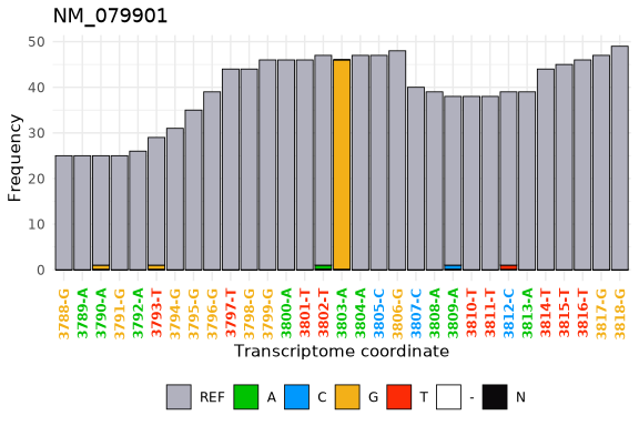
Finally, using the tx_plot_nucFreq() function we can visualize that data in the DT at an specific location.

tx_plot_nucFreq(DT, gene = "NM_079901", txRange = window_around(3803, 15))

Further documentation

The txtools user guide is available as a vignette typing vignette("txtools") at the R console.
The use cases code is available at its own repo in: https://github.com/AngelCampos/txtools_uc.

Current limitations:

Insertions: txtools is not able to deal with insertions. This is mainly because insertions are not part of the original trasncriptomic nor genomic reference space as they would alter the length of the gene model. This could be an added feature in future versions but is not a priority.
Potentially long processing times: Loading big BAM files into R commonly requires a lot of time, having this in mind txtools provides a progress bar to keep users informed about the loading status. Most importantly, depending on the ammount of both loaded reads and the size of the Gene Annotation tx_reads() processing time can take several minutes. A solution to this issue is the use of multi-threadding which has been incorporated into tx_reads() and other functions, but such functionality is only available for UNIX and MAC OS.

Additional notes:

As many R packages meant for high-throughput data analysis and manipulation, using txtools may require high ammounts of RAM memory, depending mainly on the size of BAM files being processed.