| title | author | date | output |
|---|---|---|---|
Machine Learning for Physical Activity Evaluation |
Andrew Pederson |
December 18, 2014 |
html_document |
TestURL <- "https://d396qusza40orc.cloudfront.net/predmachlearn/pml-testing.csv"
TrainURL <- "https://d396qusza40orc.cloudfront.net/predmachlearn/pml-training.csv"

download.file(TrainURL, destfile="./Training.csv", method="curl")
download.file(TestURL, destfile="./Testing.csv", method="curl")
setwd("~/Rfiles/PracticalMachineLearnProject")
TrainingBase <- read.csv("./Training.csv", na.strings=c("","NA","#DIV/0!"))
FinalTesting <- read.csv("./Testing.csv", na.strings=c("","NA","#DIV/0!"))
Some variables, like the user name and time stamps, are not necessary for our analysis and can be excluded. Others are mostly zero or NA vaules, and thus not likely worthwhile to include as predictors.
library(caret)
nsv <- nearZeroVar(TrainingBase, saveMetrics=TRUE)
na.prop <- function(x) {
      sum(is.na(x))/length(x)
  }

deletevars <- c("X","user_name","raw_timestamp_part_1","raw_timestamp_part_2"
                ,"cvtd_timestamp", "new_window", "num_window",
                rownames(nsv[nsv$zeroVar==TRUE,]),
                names(which(sapply(TrainingBase,na.prop)>0.95)))

TrainingBase <- TrainingBase[,-which(names(TrainingBase) %in% deletevars)]
To avoid overfitting our model, we split the "base" training data set 60/40 into new training and testing sets.
library(caret)
set.seed(12345)
trainIndex = createDataPartition(y=TrainingBase$classe, p = 0.60,list=FALSE)
training = TrainingBase[trainIndex,]
testingInit = TrainingBase[-trainIndex,]
There are still too many variables to plot efficiently, so we use hierarchical clustering to identify some variables of interest in the training set.
hcluster = hclust(dist(t(training[,2:52])))
plot(hcluster)
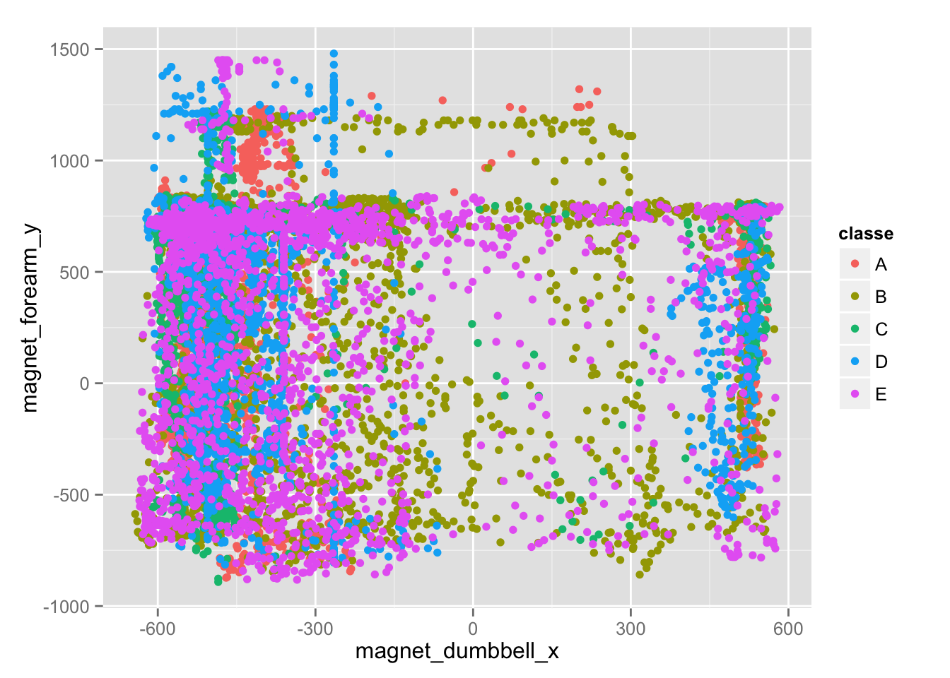
We can see that the magnetometer and accelerometer variables seem to be important in determining clustering, though it's not possible to identify any clear relationships by plotting any of those variables. The plot below illustrates how noisy this data is.
qplot(magnet_dumbbell_x, magnet_forearm_y, colour=classe, data=training)
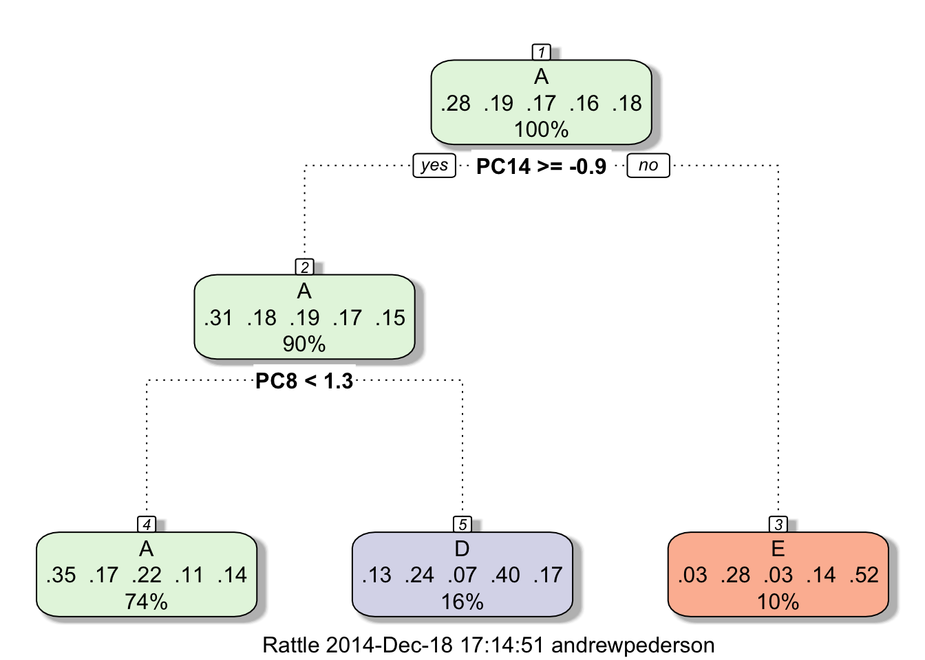
Since no clear linear relationships are visible, we decide to apply a tree-based method. An initial tree model built with the "rpart" method applied to the data preprocessed with a principle components analysis yielded less than 40% accuracy, and was not able to detect Classes B or C at all.
Prtrain <- trainControl(method="cv", number=5)
PrcompMod <- train(classe~., data=training, trControl=Prtrain, preProcess="pca", method="rpart")

library(rattle)
fancyRpartPlot(PrcompMod$finalModel)
PRpred <- predict(PrcompMod, newdata=testingInit)
confusionMatrix(PRpred, testingInit$classe)
## Confusion Matrix and Statistics
##
##           Reference
## Prediction    A    B    C    D    E
##          A 2054 1023 1264  662  796
##          B    0    0    0    0    0
##          C    0    0    0    0    0
##          D  152  288   79  513  213
##          E   26  207   25  111  433
##
## Overall Statistics
##
##                Accuracy : 0.3824
##                  95% CI : (0.3716, 0.3932)
##     No Information Rate : 0.2845
##     P-Value [Acc > NIR] : < 2.2e-16
##
##                   Kappa : 0.1709
##  Mcnemar's Test P-Value : NA
##
## Statistics by Class:
##
##                      Class: A Class: B Class: C Class: D Class: E
## Sensitivity            0.9203   0.0000   0.0000  0.39891  0.30028
## Specificity            0.3329   1.0000   1.0000  0.88841  0.94238
## Pos Pred Value         0.3542      NaN      NaN  0.41205  0.53990
## Neg Pred Value         0.9130   0.8065   0.8256  0.88290  0.85676
## Prevalence             0.2845   0.1935   0.1744  0.16391  0.18379
## Detection Rate         0.2618   0.0000   0.0000  0.06538  0.05519
## Detection Prevalence   0.7391   0.0000   0.0000  0.15868  0.10222
## Balanced Accuracy      0.6266   0.5000   0.5000  0.64366  0.62133
When we switched to a tree based method with high classification accuracy, Random Forest, however, the model worked well out of the box. Creating the model with 10 fold cross validation was computationally intensive, so the folds were reduced until they had a large effect on accuracy. 3 fold cross validation appears to be sufficient to give the model over 99% accuracy.
set.seed(625)
CV <- trainControl(method="cv",number=3, allowParallel = TRUE)
RFmodel <- train(classe ~ .,data=training,trControl=CV,method="rf", prox=FALSE)
RFmodel$finalModel
## Call:
##  randomForest(x = x, y = y, mtry = param$mtry, proximity = FALSE)
##                Type of random forest: classification
##                      Number of trees: 500
## No. of variables tried at each split: 27
##
##         OOB estimate of  error rate: 0.99%
## Confusion matrix:
##      A    B    C    D    E class.error
## A 3338    6    2    0    2 0.002986858
## B   21 2246   11    0    1 0.014480035
## C    1    8 2032   13    0 0.010710808
## D    0    0   30 1896    4 0.017616580
## E    0    2    6    9 2148 0.007852194
RFpred <- predict(RFmodel, newdata=testingInit)
confusionMatrix(RFpred, testingInit$classe)
## Confusion Matrix and Statistics
##
##           Reference
## Prediction    A    B    C    D    E
##          A 2229   10    0    0    0
##          B    3 1502    6    0    1
##          C    0    6 1358   18    3
##          D    0    0    4 1266    5
##          E    0    0    0    2 1433
##
## Overall Statistics
##
##                Accuracy : 0.9926
##                  95% CI : (0.9905, 0.9944)
##     No Information Rate : 0.2845
##     P-Value [Acc > NIR] : < 2.2e-16
##
##                   Kappa : 0.9906
##  Mcnemar's Test P-Value : NA
##
## Statistics by Class:
##
##                      Class: A Class: B Class: C Class: D Class: E
## Sensitivity            0.9987   0.9895   0.9927   0.9844   0.9938
## Specificity            0.9982   0.9984   0.9958   0.9986   0.9997
## Pos Pred Value         0.9955   0.9934   0.9805   0.9929   0.9986
## Neg Pred Value         0.9995   0.9975   0.9985   0.9970   0.9986
## Prevalence             0.2845   0.1935   0.1744   0.1639   0.1838
## Detection Rate         0.2841   0.1914   0.1731   0.1614   0.1826
## Detection Prevalence   0.2854   0.1927   0.1765   0.1625   0.1829
## Balanced Accuracy      0.9984   0.9939   0.9943   0.9915   0.9967
Accuracy is over 99% when applied to the testing dataset, and the estimated out of sample error rate is less than 1%.


