
This work focuses on implementing one of the most commonly used time-frequency decomposition tools: the Short-Time Fourier Transform (STFT). We have already extensively covered the STFT in our course summary reports, so we will not dive into the mathematical details. However, we will compare the performances of a naive implementation and one of many optimized algorithms. The naive transform is based on the direct implementation of the mathematical formula of the discrete Fourier transform. The most commonly used optimization technique is the Cooley–Tukey algorithm. We will use this fast Fourier transform to implement an accelerated version of the STFT.
The STFT algorithm lies on the Fourier transform computation over short segments of a signal to analyze. This produces the frequency spectrum on each segment which can be placed one after the other to generate a time-frequency representation. While any windowing function can be used, we will consider a rectangular window to keep our program simple and efficient. Thus, there are two main parameters to our algorithm: the window width and the number of steps between two segments. Naturally, the Fourier transform generates complex values.

Our program is implemented in C++. All signals are stored as vectors from the standard library. Besides, the complex numbers C++ library is also leverage to simplify the implementation. Finally, the STFT results are stored as a vector of complex value vectors. The behavior of the STFT is thus straightforward to implement considering a Fourier transform function Fft::dft.
See implementation
typedef std::vector<std::complex<float>> vec_complex;
typedef std::vector<float> vec_real;
typedef std::vector<vec_complex> mat_complex;

Fft::mat_complex Fft::stft_dft(Fft::vec_real &vec, size_t window_size, size_t window_step){
	Fft::mat_complex spectrogram = Fft::mat_complex();
	for (size_t begin = 0; begin < vec.size() - window_size; begin+=window_step)
	{
		spectrogram.push_back(Fft::dft(vec, begin, window_size));
	}
	return spectrogram;
}
We now need a DFT function to complete our naive STFT implementation. The kᵗʰ element of the DFT of a discrete signal xₜ of size N is defined as

Our function must iterate over each frequency step k and, in an inner loop, iterate over a time step t to perform the summation.
See implementation
Fft::vec_complex Fft::dft(const Fft::vec_complex &signal, size_t vec_begin, size_t vec_size) {
	Fft::vec_complex output;
	for (size_t k = 0; k < vec_size/2.; k++) {
		std::complex<float> sum = 0.;
		for (size_t t = 0; t < vec_size; t++) {
			float angle = 2 * PI * t * k / vec_size;
			sum += signal[t+vec_begin] * std::exp(std::complex<float>(0, -angle));
		}
		output.push_back(sum);
	}
	return output;
}
We now have a functional STFT transform. However, it is awfully slow. The time complexity of the DFT operation is O(N²). The decomposition of a ∼9s requires a computation time of 4 minutes! We will dive deeper in the results and performance later on. Although, first, let us introduce our optimization algorithm.
The computation of each term of the DFT is very close. They only differ by a complex angle in their summation. The Cooley–Tukey algorithm play with this characteristic to reduce the number of operation through the principle of dividing to conquer. The simplest form of this method is based on a binary separation, also called radix-2 decimation-in-time. Indeed, we can split our summation in an odd-indexed part and an even-indexed part of the signal, ∀ k ∈ [0, N−1],

Similarly, we can calculate, ∀ k ∈ [0, N−1],

This set of formulas is perfectly adapted to a simple recursive implementation.
See implementation
void Fft::transform_radix2(Fft::vec_complex & x) {
    int n = x.size();
    if (n == 1)
        return;

    Fft::vec_complex x_even(n / 2), x_odd(n / 2);
    for (int i = 0; 2 * i < n; i++) {
        x_even[i] = x[2*i];
        x_odd[i] = x[2*i+1];
    }
    Fft::transform_radix2(x_even);
    Fft::transform_radix2(x_odd);

    std::complex<float> w = 1.;
    std::complex<float> w_n = std::exp(std::complex<float>(0, - 2. * PI / n));
    for (int k = 0; 2 * k < n; k++) {
        x[k] = x_even[k] + w * x_odd[k];
        x[k + n/2] = x_even[k] - w * x_odd[k];
        w *= w_n;
    }
}
Note that given the algorithm's structure, the size of the input signal necessarily is a power of 2. This is not an issue given the STFT use-case. Indeed, we can easily choose an adequate window size in power of two.
This algorithm can also be implemented using in-place computation. The creation of the temporary vectors xₑ and xₒ can thus be avoided. This can heavily improve the space complexity of the program. In addition, while the time complexity O(N⋅ log(N)) theoretically remains unchanged, we would certainly observe a performance improvement as the vector creation process has linear time complexity. Finally, an in-place computation allows to calculate and store one for all the nᵗʰ roots of unity wₙ. However, the in-place implementation implies complicated operation, which we will not discuss here. For the sake of efficiency comparison, we will use this open-source in-place implementation of the radix-2 transformation.
The algorithms and partial source code presented above are all implemented as part of a simple C++ library called \textbf{Fft}. The functions defined in the associated scope are included into our main C++ file \textit{compute_spectrogram.cpp}. Besides, the open-source library AudioFile from Adam Stark is used to digest WAV files as the subject of our time-frequency analysis. The imported file sampling rate is crucial to define the temporal step and the size of the frequency bins of our time-frequency representation. However, we also have to define the window size M, and the window steps R of the representation.
We already discussed in length the uncertainty principles of the short-time Fourier transform in our course summaries. Proper window size is critical for a good representation. Wave files are usually sampled at a rate of fₛ = 44.1 kHz. After some experimentation, we found a window size of M=2¹⁰ = 1024 yields good results. The window step is arbitrarily set to half the window size R=M/2.
After computation, the absolute value of the STFT result is stored in a CSV file. The first line contains the temporal step and the frequency step of the discrete representation. A Python script then generates a proper spectrogram visualization from the data provided through the CSV file. The whole process is streamlined using a makefile which allows using a single command to generate a spectrogram. From the main directory,
make file=./audio\_files/my\_audio.wav
We can now test and compare our three algorithms on several audio files available in ./audio_files. All audio files are encoded on 32-bit float at a sampling rate of 41.1 kHz. We have selected a human natural speech sample, a couple of electronic pieces of music with specific characteristics, and a nature audio recording of birds.
The spectrograms shown below are produced using our FFT algorithm (out-of-place computation). However, the spectrogram representation is (fortunately) strictly independent to the Fourier transform algorithm used. Still, all spectrogram produced during this study are available in ./spectrograms
-
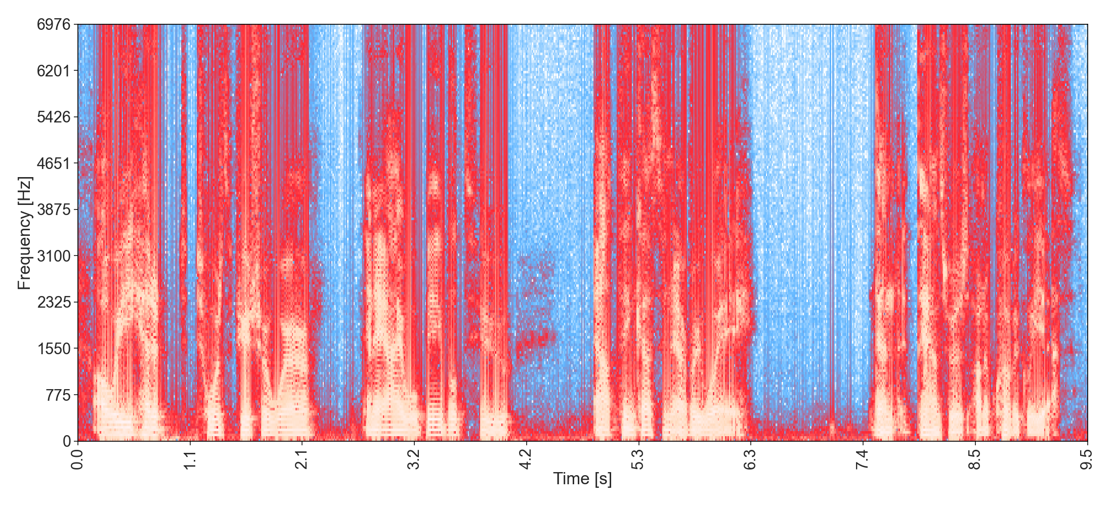
"Are we headed towards a future where an AI will be able to out-think us in every way? Then the answer is unequivocally yes." - Elon Musk
The time-frequency analysis of natural language speech is one of the most powerful techniques for transcription. Heavy work is currently put into the application of CNN on such representation. We will dive deeper into this technique in our research project.
-
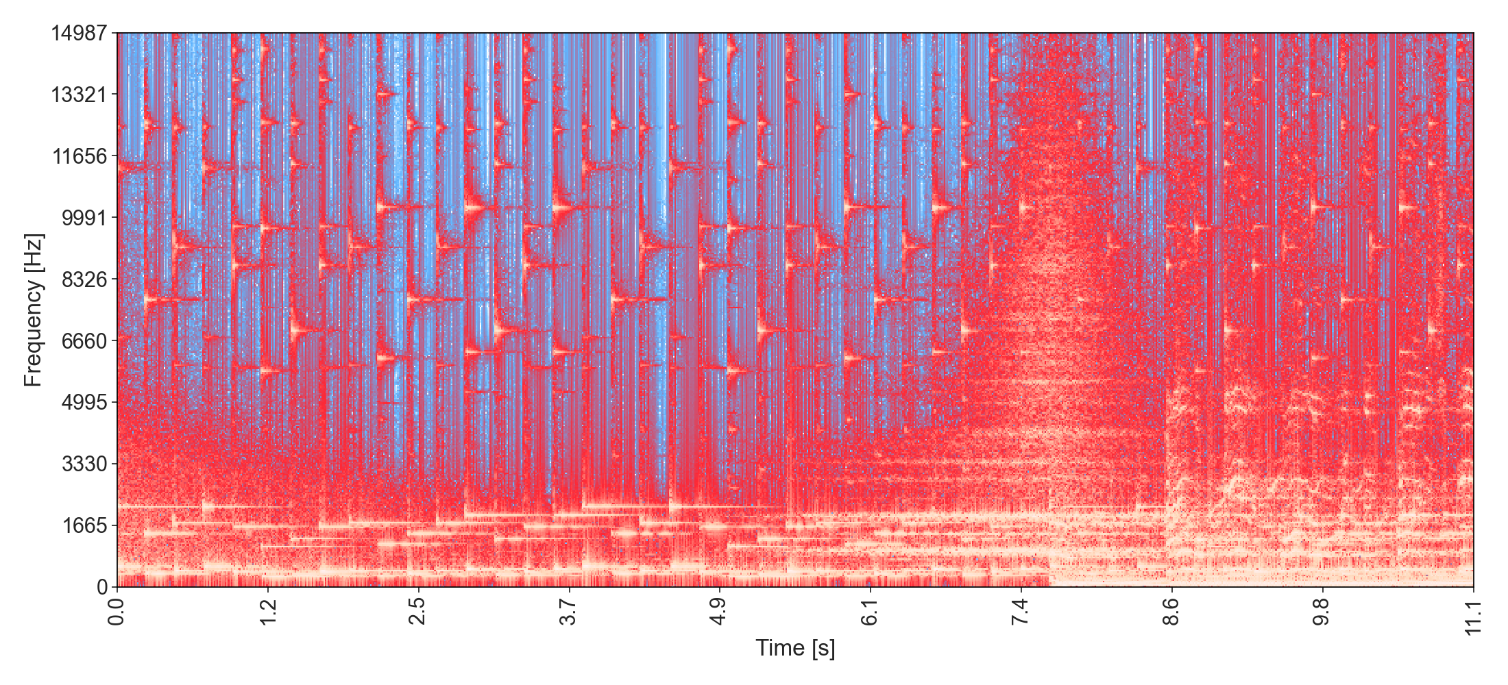
Introduction of the song All Around The Roses from SAINtJHN:
This xylophone sample perfectly illustrates the use of the time-frequency representation to decompose music instruments notes in a fundamental frequency and all the harmonics that compose its timbre.
-
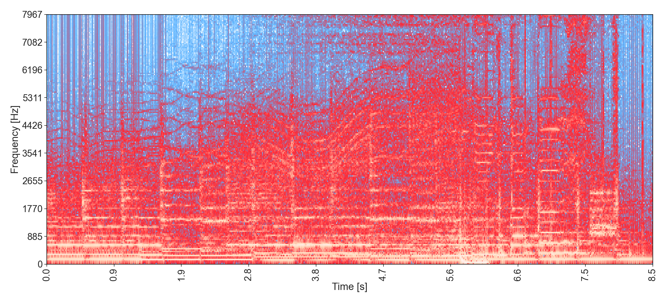
Introduction of the song Sacrificial from Rezz:
We can observe the frequency crescendo of this song until the introductory drop around 5s.
-
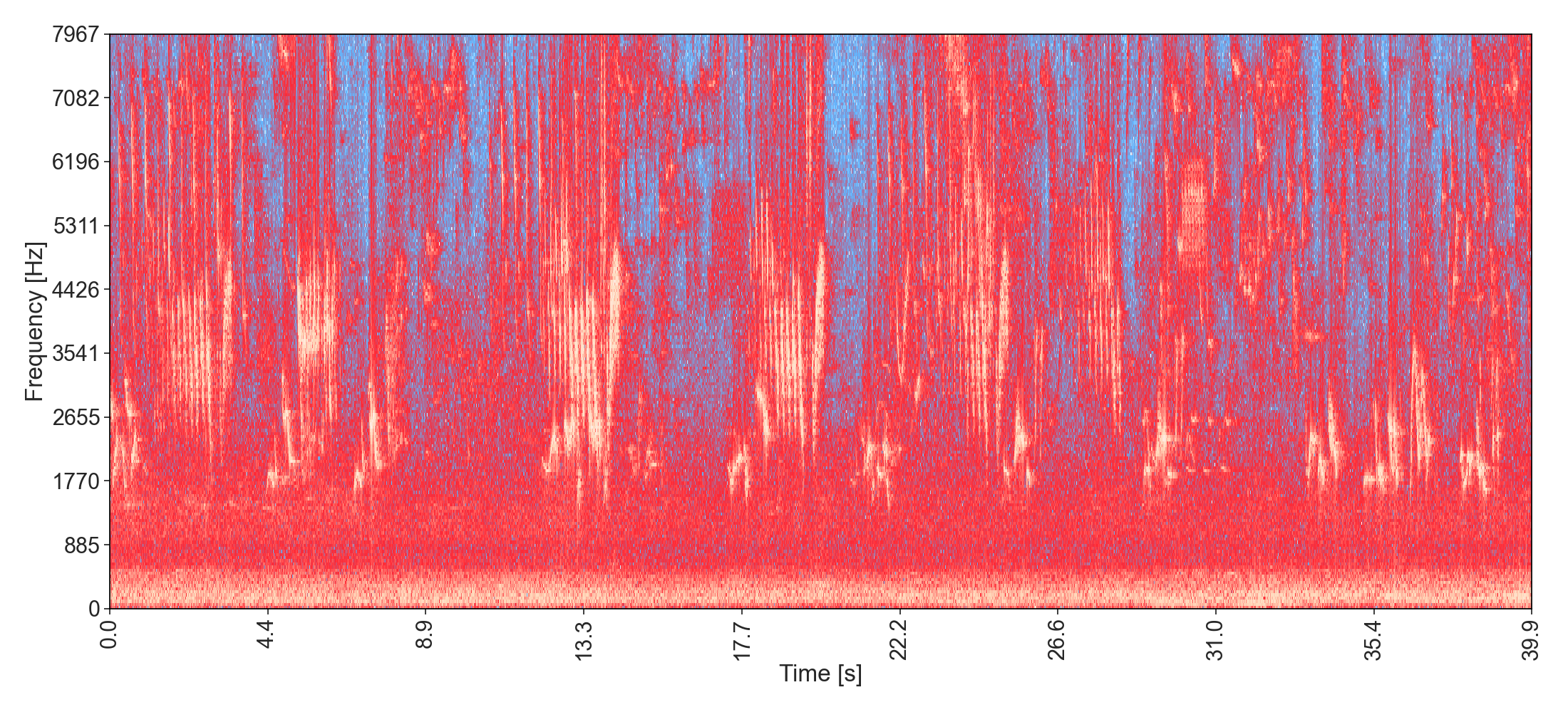
Bird Sounds Spectacular : Morning Bird Song from Paul Dinning - Wildlife in Cornwall:
Multiple birds and background noise of nearby rad traffic can be heard simultaneously in this sample. Nevertheless, we can identify patterns associated with specific bird songs. Most notably, one is repeated at 13s and 18s. The road noise is contained in the lower frequency range.


| FFT in-place | FFT out-of-place | DFT | |
|---|---|---|---|
| SAINtJHN - All Around The Roses (11s) | 313 | 853 | 60913 |
| Rezz - Sacrificial (8s) | 241 | 648 | 46159 |
| Morning Bird Song (39s) | 1152 | 3069 | 2178394 |
| Elon Musk about Consciousness | AI (9s) | 268 | 739 | 52204 |
As expected, the radix-2 algorithm allows a way faster computation. Given the better time complexity, the execution time reduction factor is proportional to the logarithm of the analyzed signal's length. Finally, we can note that the gain in performance due to the in-place computation is significant. It reduces the execution time of a factor of 3 in comparison to the out-of-place algorithm.