This repository contains a collections of data structures and algorithms from the Manning book Algorithms and Data Structures in Action-
You can buy the book on Manning's web site: https://www.manning.com/books/algorithms-and-data-structures-in-action
The book explains these data structures using pseudo-code, because we wanted to highlight the logic of the algorithms rather than having to focus on the implementation details intrinsic to any programming language.
At the same time, hands-on learning is also an important part of the teaching process, so we gathered here a collection of implementations of those same algorithms, using a few different programming languages.
For each data structure, you can find the link(s) to the livebook Manning's website, where you can take a quick look at the material and preview the book.
Here you can read more about the structure and content of the book: feel free to take a look and decide if it's the right algorithms book for you.
To have a taste of how the book is structured, you can also read this free excerpt from chapter 1, discussing the process of designing an algorithm by progressively solving the "knapsack problem".
| Chapter 2 | Java | JavaScript | Python | Jupyter Notebook (profiling) |
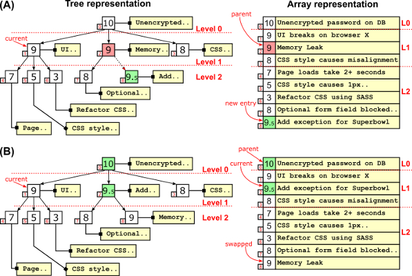
A heap is conceptually a tree, but it’s implemented using an array for the sake of efficiency. While regular heaps are binary balanced trees, d-ary heaps use d-ary trees, reducing the tree's height. Depending on what operations are performed more frequently on the heap, a larger branching factor can provide a significant speed-up.
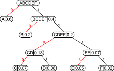
Huffman's algorithm is probably the most famous data compression algorithm: a simple, brilliant greedy algorithm that, despite not being the state of the art for compression anymore, was a major breakthrough in the '50s.
A Huffman code is a tree, built bottom up, starting with the list of different characters appearing in a text and their frequency. The algorithm iteratively:
- selects and removes the two elements in the list with the smallest frequency
- then creates a new node by combining them (summing the two frequencies)
- and finally adds back the new node to the list.
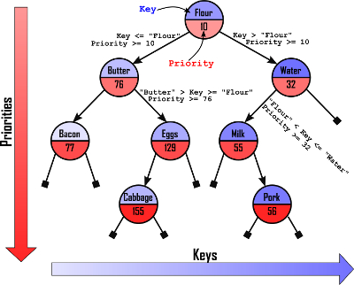
Treap is the portmanteau of tree and heap: binary search trees, in fact, offer the best average performance across all standard operations: insert, remove and search (and also min and max). Heaps, on the other hand, allow to efficiently keep track of priorities using a tree-like structure. Treaps merge the characteristics of these two data strucures to get the best of both.
| Chapter 4 | JavaScript |
Bloom filters work like sets, storing entries and allowing fast lookup. In exchange of a (tunable) ratio of false positives, they allow to store large sets using only a constant number of bits per key (while hash-tables, for instance, would require space proportional to the size of the keys).
| Chapter 5 | JavaScript |
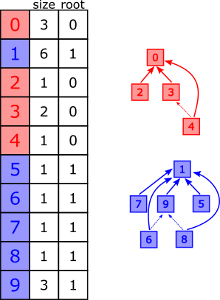
We use a disjoint-set every time that, starting with a set of objects, we would like to account for the partitioning of this set into disjoint groups (i.e. sub-sets without any element in common between them).
| Chapter 6 | Java (in progress) | JavaScript |
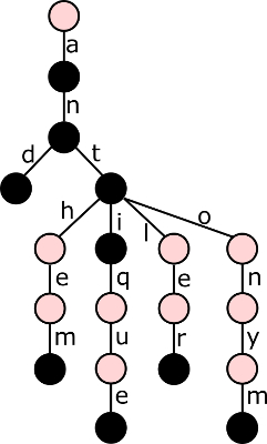
This data structure allows to more efficiently store and query large sets of strings, assuming many of them share some common prefixes. Many applications manipulating strings can benefit from using trie, from spell-checkers to bioinformatics.
| Chapter 6 | Java (in progress) | JavaScript |
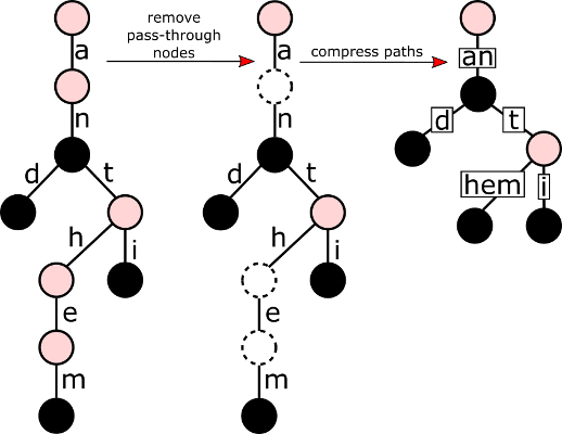
Storing tries can be cheaper than holding these values in binary search trees or hash tables, but it can require a lot of memory. Radix tries compress paths, whenever possible, to provide a more compact representation of these tries, without having to compromise interms of complexity or performance.
| JavaScript |
The Needleman–Wunsch algorithm is an algorithm used in bioinformatics to align protein or nucleotide sequences.
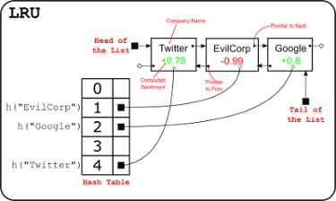
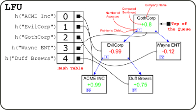
Thread safe implementations of LRU and LFU caches: a data structure that is vital at many levels of internet-based applications, allowing to remember recently (or frequently) seen data and the saving remote call, or expensive computation, that would be needed to retrieve those data again.
| Chapter 9 | JavaScript |
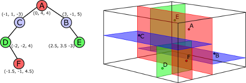
K-d trees are an advanced data structure that helps performing spatial queries (nearest neighbor search and intersections with spherical or rectangular regions) more efficiently. K-d trees are great with low-and medium-dimensional spaces, but suffer sparsity of high-dimensional spaces; they also work better on static datasets, because we can build balanced trees on construction, but insert and remove are not self-balancing operations.
| Chapter 10 | JavaScript |
To overcome the issues with k-d trees, alternative data structures like R-trees and Ss-trees have been introduced.
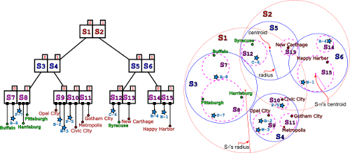
Ss+-trees cluster data in overalpping hyperspheres, using a few heuristics to maintain the tree as balanced as possible.
Although none of these structures can offer any guarantee on the worst-case running time, in practice they perform better than k-d trees in many situations, and especially for higher-dimensional data.
| Chapter 12 | Chapter 13 (MapReduce) | Python | Jupyter notebook (demo) | Jupyter Notebook (profiling) |
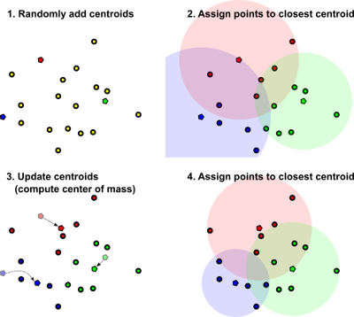
k-means is the simplest and oldest clustering algorithm; it partitions data in a pre-determined number of spherical clusters.
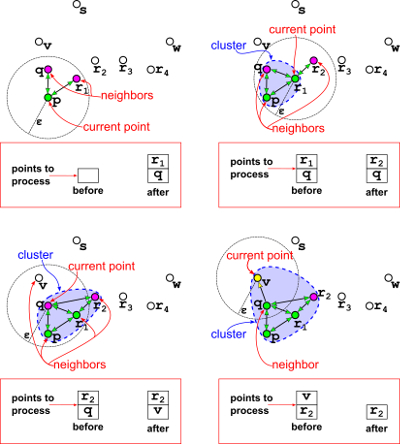
DBSCAN is an acronym for “Density-based spatial clustering of applications with noise”, and the main difference in the approach with respect to k-means is already clear from its name: while k-means is a centroid-based algorithm, and as such builds clusters as convex sets around points elected as centroids, a density-based algorithm defines clusters as sets of points that are close to each other, close enough that the density of points in any area of a cluster is above a certain threshold.
| Chapter 12 | Python | Jupyter notebook |
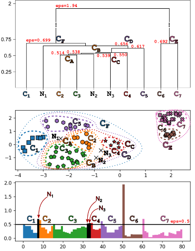
The idea behind OPTICS is that the order in which points are processed does matter, and in particular it can make sense to keep expanding a “frontier” for current cluster by adding the unprocessed point that is closest to the cluster (if it is reachable from the cluster).
| Chapter 13 |
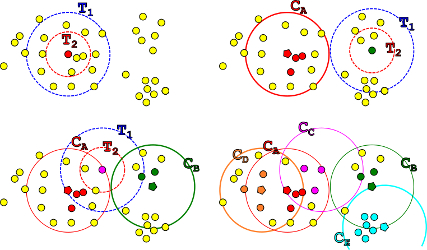
Canopy clustering groups points into spherical regions (circles in our 2D examples), like k-means, but unlike it, these regions can overlap, and most points are assigned to more than one region.
The canopy clustering algorithm is faster and simpler than k-means, as it runs in a single pass, doesn’t have to compute the centroids for the canopies (spherical pseudo-clusters), and doesn’t compare each point to each centroid; instead, it elects one point in the dataset as the center of each canopy, and adds points around it to the canopy.
| Chapter 14 | Java | JavaScript: JsGraphs lib |
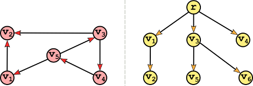
A graph G=(V,E) is usually defined in terms of two sets:
- A set of vertices
V: independent, distinct entities that can appear in any multiplicity. A graph can have 1, 2, 100 or any number of vertices but, in general, graphs don’t support duplicate vertices. - A set of edges
Econnecting vertices: an edge is a pair of vertices, the first one usually denoted as the source vertex, and the second one called the destination vertex.
Graphs are very similar to trees. They are both made of entities (vertices/nodes) connected by relations (edges), with a couple of differences:
- In trees, vertices are usually called nodes;
- In trees edges are somehow implicit: since they can only go from a node to its children, it’s more common to talk about parent/children relations than explicitly list edges. Also, because of this, trees are implicitly represented with adjacency lists.
Furthermore, trees have other peculiar characteristics that makes them a strict subset of the whole set of graphs; in particular, any tree is a simple, undirected, connected and acyclic graph.
