1 - Workflow
2 - Getting started
2.1 - Technical Notes
2.2 - Main widget: "File" tab
2.3 - Main widget: "Advanced" tab
2.4 - Main widget: Config droplists and "Process Data!" button
3 - Data Processing
3.1 - Treatment configuration
3.2 - Run calculations
3.3 - Load specific configurations
3.4 - Tools: Precision and Non-Linearity experiment
3.5 - Diagnostics and report
IAU_DataProc can analyse measurement series that have been analysed in IAU_Chrom. Prerequisite: A relative calibration scheme, i.e. a sequence of calibration and sample measurements. The following list describes the workflow in IAU_DataProc; Fig. 1 on the next page shows the interplay of IAU_Chrom and IAU_DataProc.
- Load IAU_Chrom data. Input are results generated with IAU_Chrom, i.e. integration of chromatographic signals (signal area, height etc.). Sect. 2.
- Add the measurement sequence. IAU_Chrom results do not contain information on what was measured in what sequence. Add this info for further analysis. Sect. 2.
- Define sample and calibration treatment. Calibration, i.e. interpolation of calibration points, can be done in various ways, i.e. point-2-point, curve fitting etc. Sect. 3.
- Run calculations and have a look. Use results plot and results table features to display results. Sect. 3.
- Save results in IDL binary format. Allows you to continue working on the experiment later on. Results can also be saved as text-files. Sect. 3.
- Specific tools for specific experiment types: Analyse Precision and Non-Linearity experiments with specific tools. Sect. 3.
The core features of IAU_DataProc can be scripted: Settings for the evaluation of multiple experiment can be put into a csv-table and called from the IAU_DataProc main widget. Based on this scripting feature, an experiment database can be created.
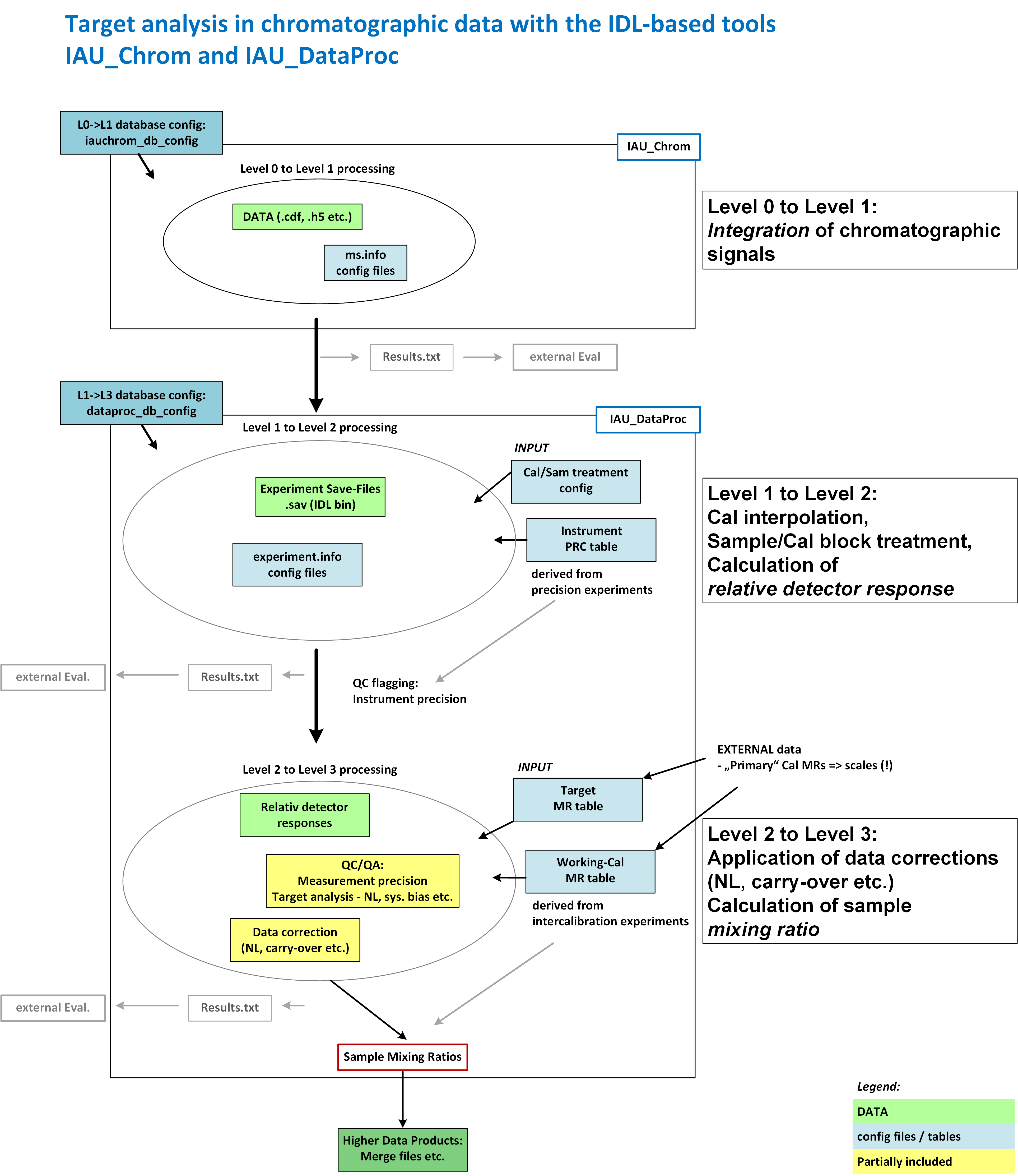
Fig. 1 - Interaction of IAU_Chrom and IAU_DataProc. Right side of the schematic: processing step, left side: software implementation
- Compatibility. IAU_DataProc is written in the IDL programming language on and for Windows machines (Win 7). A version for Unix-based systems does not exist. Windows 10 can cause problems with the plot windows (lagging etc. but no crash).
- Error handling is implemented which avoids total crashes in most cases. To avoid data loss in any case, save your progress regularly.
- To use IAU_ DataProc on the system partition on your Windows machine (C:\), it might be necessary to run IDL or the IDL virtual machine in administrator mode.
- To use the code version (not pre-compiled), an IDL installation (v8.4 or greater) is required.
Start IAU_DataProc:
- Runtime version, virtual machine only: run IAU_DataProc_v1...exe;
- Code version, IDL installed: open and run the IAU_DataProc _v1...pro from the root directory of the IAU_DataProc project.
Starting IAU_DataProc opens the main widget, shown in Fig. 2.
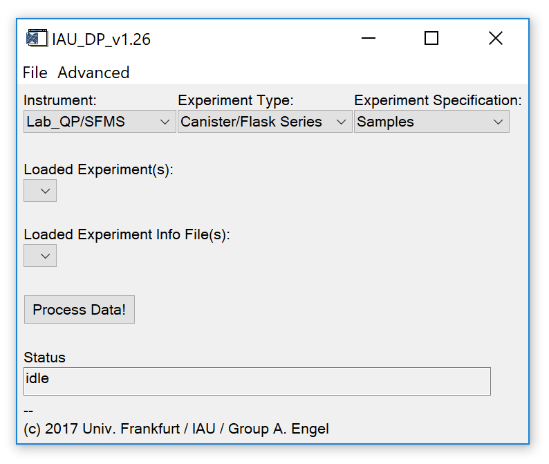
Fig. 2 - Main widget.
All further widgets (plots, tools) appear as soon as called/required.
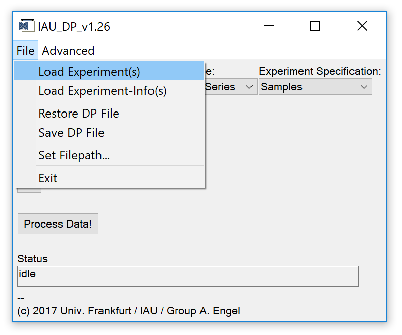
Fig. 3 - File tab on main widget.
'File' 'Load Experiment(s)': Load an IAU_Chrom experiment, i.e. the IDL binary file that can be created in IAU_Chrom with 'File' 'Save Experiment' on the IAU_Chrom main widget (*chrom.sav). The loaded experiment(s) should of course contain signal integration results. Multiple *chrom.sav files can be loaded.
'File' 'Load Experiment-Info(s)': Load an experiment info file, i.e. a text/csv file that contains information about the measurement sequence of the loaded IAU_Chrom experiment. If multiple IAU_Chrom save files were loaded, multiple experiment info files have to be loaded accordingly.
'File' 'Restore DP File': Restore a processed /saved experiment. Expected file name extension is *dp_data.dat. A configuration file with extension *dp_expcfg.dat is also expected to be in the same directory (automatically created if the 'save dp file' routine is called).
'File' 'Save DP File': Save the current experiment including configuration and results to and IDL binary file. Two files are created; results are stored in *dp_data.dat, configuration is stored in *dp_expcfg.dat. If multiple IAU_Chrom experiments were loaded / processed, IAU_DataProc results will be combined to a single save file.
'File' 'Set Filepath...': Set the default directory where to look for save files etc.
'File' 'Exit': Exit the program and close all widgets. Plot and table widgets may stay open and have to be closed manually.
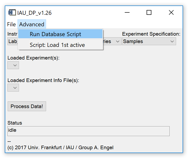
Fig. 4 - Advanced tab on main widget.
'Advanced' 'Run Database Script': Run a database script to process multiple experiments automatically.
'Advanced' 'Script: Load 1st active': Load the first experiment (and configuration) that is set to active (active flag = 1) from a database script.
Find a detailed explanation how to configure the database script in the header of the example script table header.
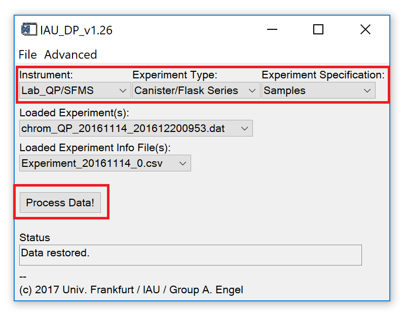
Fig. 5 - main widget options.
After experiment(s) and experiment info file(s) have been loaded (or a save file was restored), the droplists marked in Fig. 5 (upper part) should be set to appropriate selections.
- Instrument: Should automatically be set to the correct value based on the information stored in the IAU_Chrom save file. Correct manually if necessary.
- Experiment Type: Select "Canister/Flask Series" if each sample was analysed in a block of repeated measurements of the same sample. Select "In situ/Continuous" if multiple samples were analysed in one block (between calibration measurements).
- Experiment Specification: Unused feature. Leave at default selection ("Samples").
Press the "Process Data!" button (Fig. 5, lower part) to call the data processing widget (Fig. 6, next section).
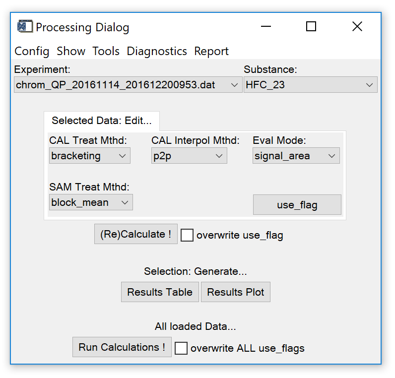
Fig. 6 - data processing widget. Droplist selectsion in the "edit..." section resemble the current evaluation settings for the selected species in the selected experiment.
Fig. 6 shows the processing widget (dialog). There are different ways how to proceed with analysing the data. In principle, each species found in the IAU_Chrom experiment(s) can be evaluated with a specific treatment configuration, i.e. treatment of calibration measurements, interpolation of the calibration points and treatment of the sample measurements (Fig. 6, "Edit..." section in the centre).
[] Treatment of calibration measurements. Determines which calibration measurements or blocks of measurements are considered as "calibration points".
- CAL Treat Mthd: bracketing. Default. Only calibration measurements before and after sample measurements (blocks) are used. If three or more calibration measurements are found between sample measurements, those that do not directly bracket the sample measurements are discarded.
- CAL Treat Mthd: block_mean. The mean of each block of calibration measurements is used.
- CAL Treat Mthd: preceding. Only calibration measurements directly before each sample measurement (block) are used.
[] Interpolation of calibration points. Sets the method for the temporal interpolation of the calibration points to where the samples were measured.
- CAL interpol Mthd: p2p. Default. Interpolation is done from "point to point", i.e from one calibration point to the next.
- CAL interpol Mthd: calsmean. The mean detector response of all calibration points is used (no interpolation).
- CAL interpol Mthd: lin_fit. A linear fit is calculated for the calibration points.
- CAL interpol Mthd: polyfit_dg2. A polynomial fit (2^nd^ degree) is calculated for the calibration points.
[] Treatment of sample measurements. Determines which sample measurements are used, which are discarded and how blocks of measurements are treated.
- SAM treat Mthd: block_mean. Default. For each block of sample measurements, the mean detector relative to the interpolated calibration point (relative response, rR) is calculated. Do not use if multiple different samples are measured within one block (use "individual" in that case).
- SAM treat Mthd: individual. Use if multiple samples are measured within one block, e.g. in case of continuous sampling. An individual relative response is calculated for each sample measurement.
- SAM treat Mthd: block_last... . Only the last ... measurements of a sample block are used. Mean relative response is calculated from the remaining measurements. Can be useful to discard measurement affected by carry-over.
[] Eval Mode. IAU_Chrom integration results contain signal area and signal height. Signal area is the default selection; change to signal height if a species should be evaluated with height data.
[] Use Flag. Opens an editable table, see Fig. 7 red box. By setting the use_flag of a measurement to zero (enter a "0" in the use_flag column and press [enter]), the respective measurement can be excluded from further evaluation. To apply a changed use_flag, re-run calculations by pressing the (Re)Calculate !" button (see also sect. 3.2). If you want to undo this operation (re-include the measurement), enter a "1" in the use_flag column, press [enter] and recalculate.
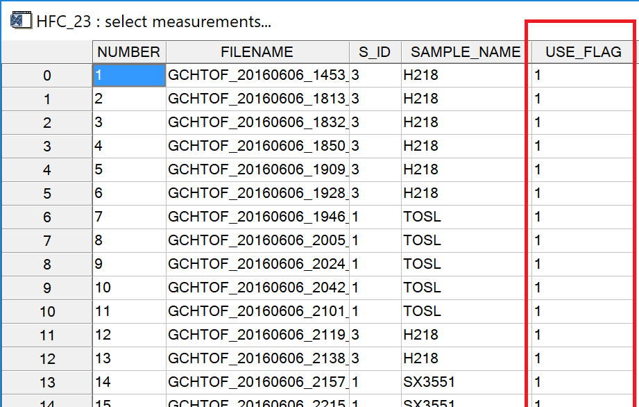
Fig. 7 - "edit use_flag" table. Changes to other columns than the use_flag column have no effect.
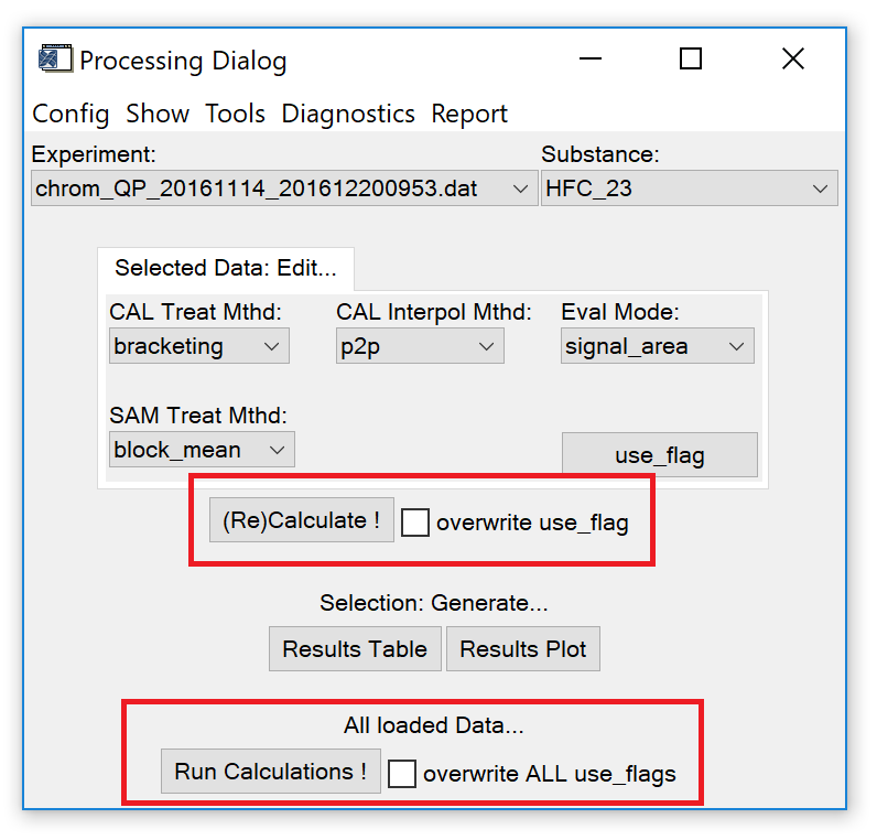
Fig. 8 -- data processing widget, "run calculations".
"(Re)Calculate !" button. Use this option to calculate results for the selected species in the selected experiment or after the treatment configuration has been changed. If calculations were done before for other species, their results will not be recalculated.
"overwrite use_flag" checkbox. Activate to reset the use_flag of all measurements for the selected species and experiment to the default value specified in the experiment info file. This change is only applied if the "(Re)Calculate !" button is pressed.
All loaded data: "Run Calculations !" button. Calculate results for all species in all loaded experiments. The current selection of treatment configuration (see sect. 3.1) is used.
All loaded data: "overwrite ALL use_flags" checkbox. If activated, the use_flag is reset to the default value (specified in experiment info file) for all measurements. This change is only applied if the "Run Calculations !" button is pressed.

Fig. 9 - data processing widget, 'config' tab.
The config menu on the processing dialog allows you to load additional information for the experiment. This information will also be stored in the save file that can be created from the main widget.
- Precision Table. A table containing reference measurement precision values for each species measured with an instrument. Precision values are used to plot error bars on the results plot (Fig. 16) and calculate the precision flag shown in the results table (Fig. 17).
- CAL Mixing Ratio Table. A table containing mixing ratios attributed to species found in the calibration gas used. If loaded, mixing ratios will be calculated and displayed in the results table (Fig. 17). Note that this calculation assumes linear proportionality of calibration and sample detector response.
- TGT Mixing Ratio Table. A table containing mixing ratios attributed to species found in the target gas(es) measured with in the experiment. Necessary if the NL analyser tool should be used to calculate a detector non-linearity correction function (see sect. 3.4).
- Treat. Config. A table containing species-specific treatment configurations (see sect. 3.1). Avoids the manual selection of the treatment config for each species and is especially useful if different species should be evaluated with different treatment configs.
All configuration data/settings can be removed from the experiment by using the "Config → Reset → ..." function. The treatment configuration can also be exported by using the "Config → Export Treat. Config" function.
To see if and which configuration has been loaded, use the functions from the show-tab on the processing dialog (Fig. 10).
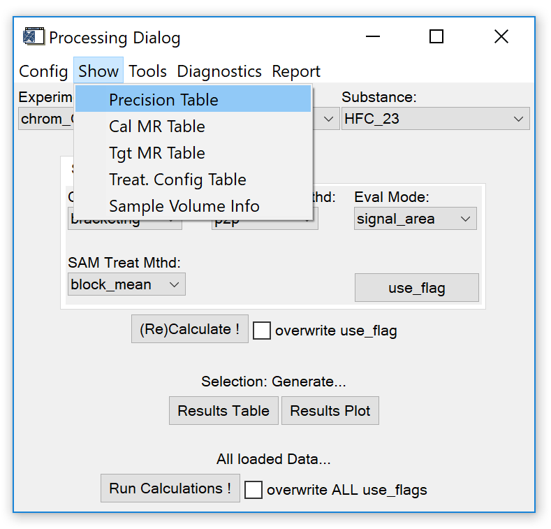
Fig. 10 - data processing widget, 'show' tab.
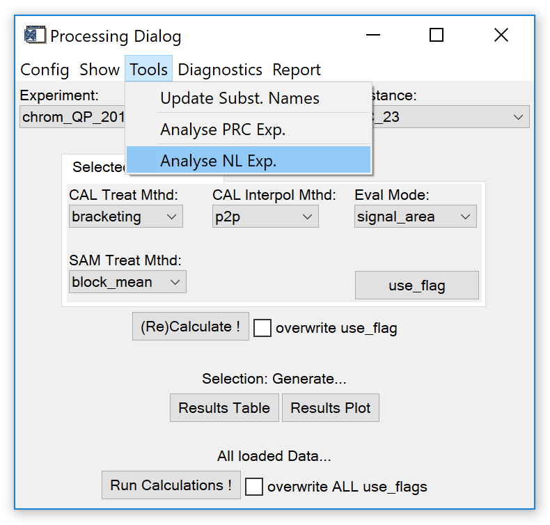
Fig. 11 - data processing widget, 'tools' tab.
Update Subst. Names. Load a species name definition list. Useful e.g. if different names (spelling etc.) were used for the same species. Unambiguous species names are crucial since configuration data (Cal mixing ratio etc.) is selected based on the species' name.
Analyse PRC Exp. Calls a widget (Fig. 12) to analyse a precision experiment, i.e. a measurement series that only contains measurements of the same reference gas.
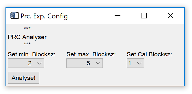
Fig. 12 - Precision experiment analyser widget.
Minimum and maximum block size ("blocksz") refer to the number of sample measurement in a row in between calibration measurements. At least two measurements are required to calculate a relative standard deviation, which is why the minimum value is a block size of two. The maximum block size is dependent on the number of measurements of the reference gas (precision experiment). Calibration block size can be set to 1, 2 or 3.
Trigger the calculation by pressing the "Analyse" button. After calculations are done, a file dialog pops up. It requires you to select a folder where to save results. For each species defined in the experiment, a text file with results will be created in the selected folder. Each file contains results (relative detector response and block relative standard deviation) for the selected block size range.
Analyse NL Exp. Calls a widget (Fig. 13) to analyse a non-linearity experiment, i.e. a series of measurements of target gases with known mixing ratios.
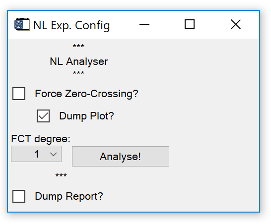
Fig. 13 - Non-linearity experiment analyser widget.
Requires: Target gases measured in the measurement sequence and target mixing ratios loaded (see sect. 3.3)
Mode 0: No calibration gas mixing ratios loaded estimation of calibration gas mixing ratios.
Mode 1: Calibration gas mixing ratios loaded fitting a non-linearity correction curve.
**
**
Options:
- Force Zero-Crossing. Check this box to force the non-linearity correction function through zero, i.e. x/response = 0, y/mixing ratio = 0. Only use with NL analyser mode 1.
- Dump Plot. Check this box to cause a results plot to appear after calculations are finished.
- FCT degree. Degree of the polynomial that is fitted. Select an appropriate value (1-4) depending on how many different target mixing ratios were measured.
- Dump Report. Check this box to save results to a text file after calculations are finished.
Press the "Analyse" button to call the calculation. If the show plot checkbox is checked, one of the following plots appear:
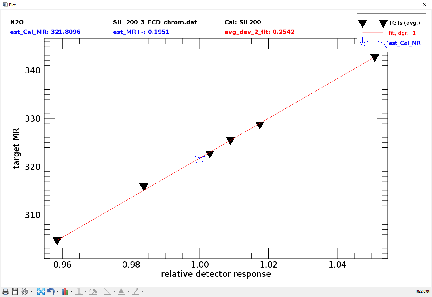
Fig. 14 - NL analyser tool in mode 0, calibration gas mixing ratio estimation. X-axis: relative detector response (sample/cal), y-axis target mixing ratios (from definition file, see sect. 3.3).
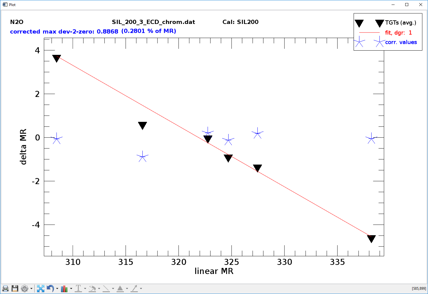
Fig. 15 - NL analyser tool mode 1, non-linearity correction function. X-axis: mixing ratio calculated by linear proportionality, y-axis: difference of mixing ratio calculated by linear proportionality minus the specified target mixing ratio (from definition file, see sect. 3.3). Black triangles: values before correction, blue asterisks: values after correction.
Note that you can only execute calculations for the species currently selected on the processing dialog (Fig. 6).
To have a look at your results, press the "Results Table" or "Results Plot" button. This opens a table widget / plot with results for the selected species in the selected experiment (Fig. 16 and Fig. 17).
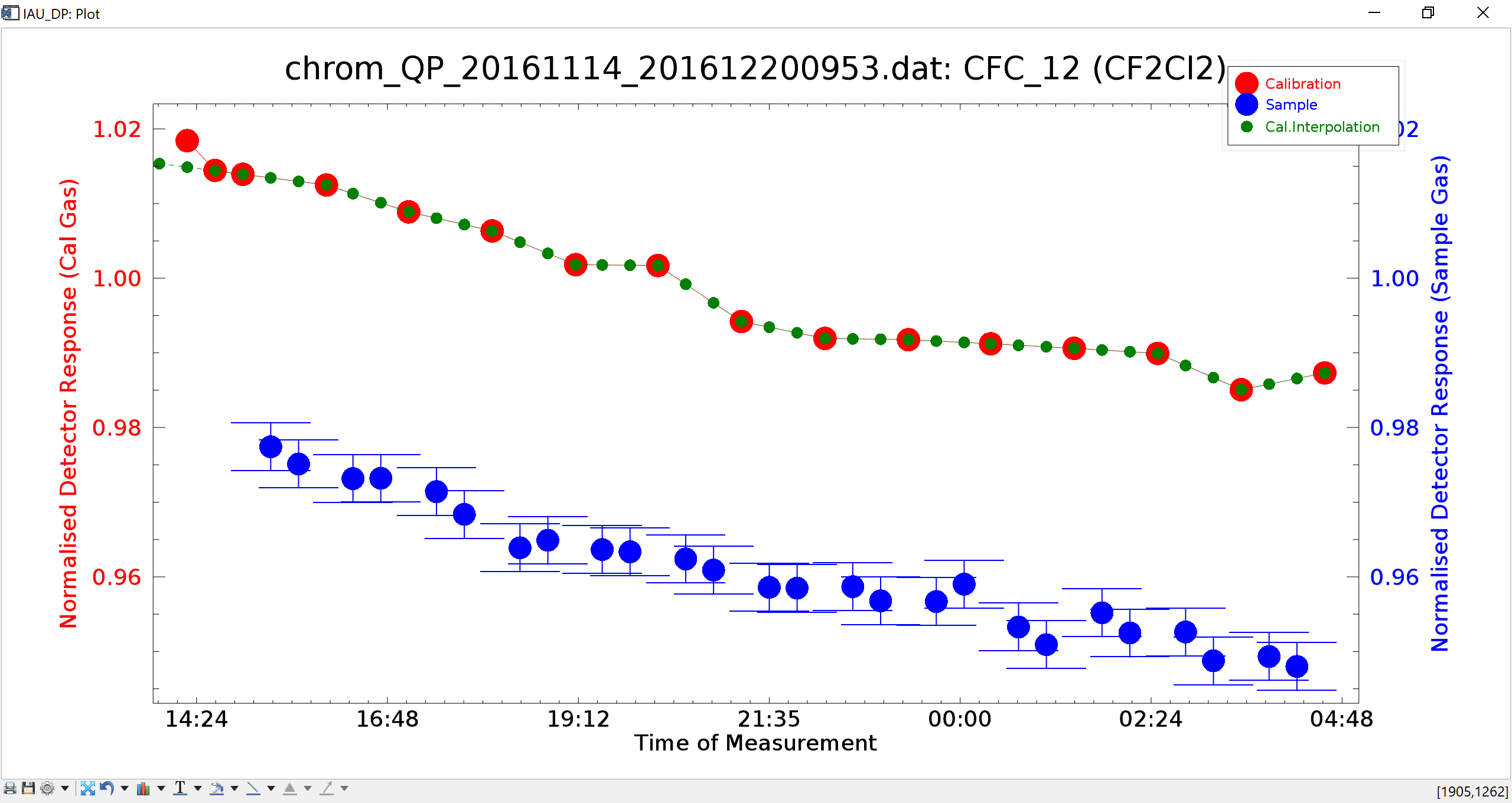
Fig. 16 - Results plot. Error bars for sample measurements only display if an instrument precision table has been loaded.
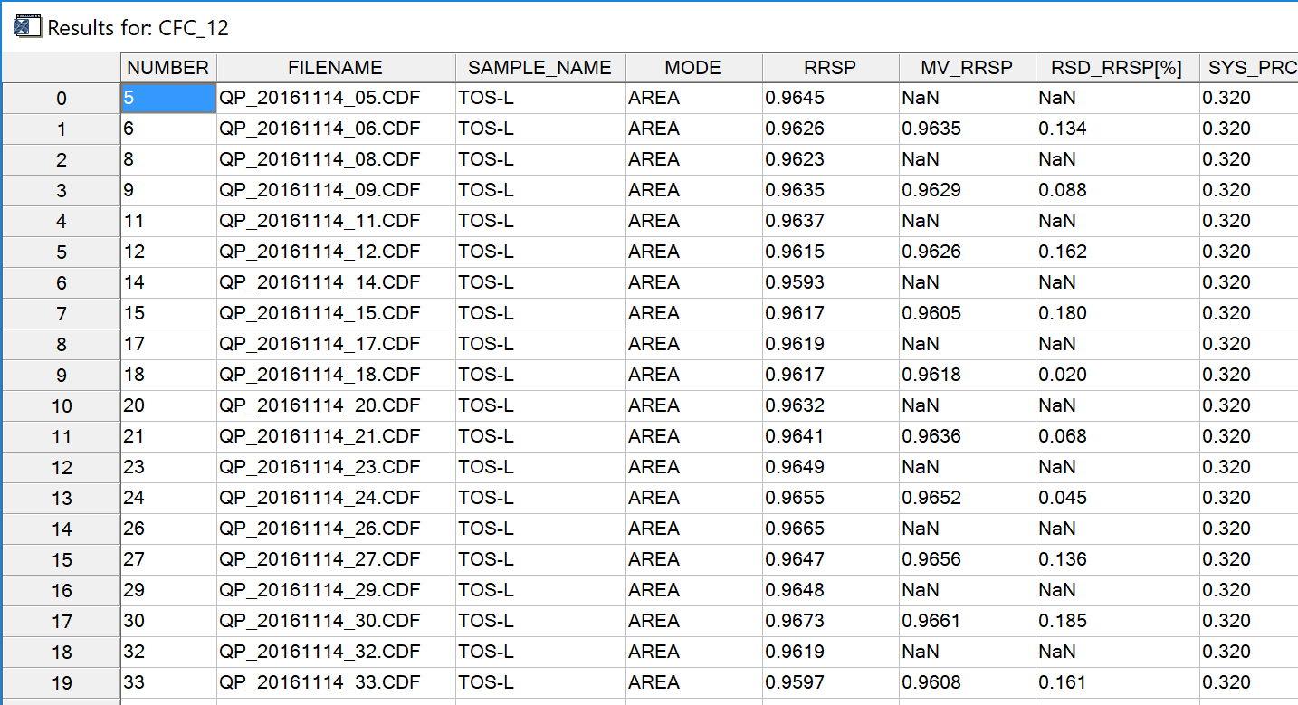
Fig. 17 - Results table. Call a more detailed version from the diagnostics menu (see Fig. 18).
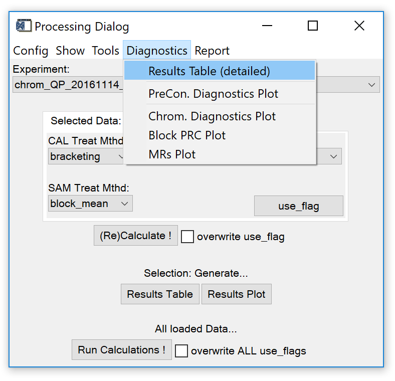
Fig. 18 - Data processing widget, 'diagnostics' tab.
From the diagnostics menu, you can also call diagnostic plots with chromatographic ("Chrom. Diagnostics Plot") and sample preconcentration data ("PreCon. Diagnostics Plot") if available.
The "Block PRC Plot" function calls a plot that shows the relative standard deviations of all sample blocks.
If calibration gas mixing ratios have been loaded (see sect. 3.3), a plot that shows sample mixing ratios can be called with the "MRs Plot" function.
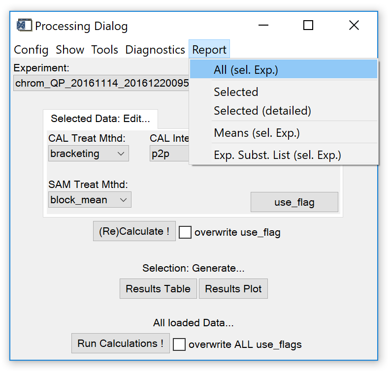
Fig. 19 - Data processing widget, 'report' tab.
From the report tab of the processing dialog, you can create different report files:
- All (sel. Exp.). Creates report files for all species of the selected experiment. The name of the report file indicates the species.
- Selected. Create a report file for the selected species of the selected experiment. The name of the report file indicates the species.
- Selected (detailed). Same as "selected" but contains information that is more detailed.
- Means (sel. Exp.). Creates a report file with average results for all species in the selected experiment.
- Exp. Subst. List (sel. Exp.). Creates a report file containing results for specific species. Requires a species list to be loaded.