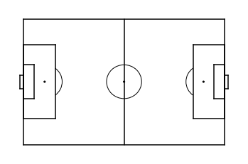
This is a package to visualize soccer data
To install it simply
pip install matplotsoccer
You can also:
- plot a green field with white lines instead of a white field with black lines
- adjust the figure size
- add a scatterplot
- reactivate the axis.
matplotsoccer.field("green",figsize=8, show=False)
plt.scatter(x,y)
plt.axis("on")
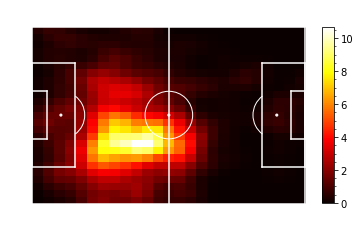
plt.show()hm = matplotsoccer.count(x,y,n=25,m=25) # Construct a 25x25 heatmap from x,y-coordinates
hm = scipy.ndimage.gaussian_filter(hm,1) # blur the heatmap
matplotsoccer.heatmap(hm) # plot the heatmapThe most important parameters are:
- the color map (any color map accepted by matplotlib will work)
- the color of the field lines
- adding a colorbar to the right of the heatmap
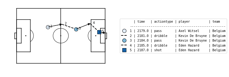
matplotsoccer.heatmap(hm,cmap="hot",linecolor="white",cbar=True)Here is an example of five actions in the SPADL format (see https://github.com/ML-KULeuven/socceraction) leading up to Belgium's second goal against England in the third place play-off in the 2018 FIFA world cup.
| game_id | period_id | seconds | team | player | start_x | start_y | end_x | end_y | actiontype | result | bodypart |
|---|---|---|---|---|---|---|---|---|---|---|---|
| 8657 | 2 | 2179 | Belgium | Axel Witsel | 37.1 | 44.8 | 53.8 | 48.2 | pass | success | foot |
| 8657 | 2 | 2181 | Belgium | Kevin De Bruyne | 53.8 | 48.2 | 70.6 | 42.2 | dribble | success | foot |
| 8657 | 2 | 2184 | Belgium | Kevin De Bruyne | 70.6 | 42.2 | 87.4 | 49.1 | pass | success | foot |
| 8657 | 2 | 2185 | Belgium | Eden Hazard | 87.4 | 49.1 | 97.9 | 38.7 | dribble | success | foot |
| 8657 | 2 | 2187 | Belgium | Eden Hazard | 97.9 | 38.7 | 105 | 37.4 | shot | success | foot |
Here is the phase visualized using matplotsoccer.actions()
matplotsoccer.actions(
    location=actions[["start_x", "start_y", "end_x", "end_y"]],
    action_type=actions.type_name,
    team=actions.team_name,
    result= actions.result_name == "success",
    label=actions[["time_seconds", "type_name", "player_name", "team_name"]],
    labeltitle=["time","actiontype","player","team"],
    zoom=False
)
(c) Tom Decroos 2019


