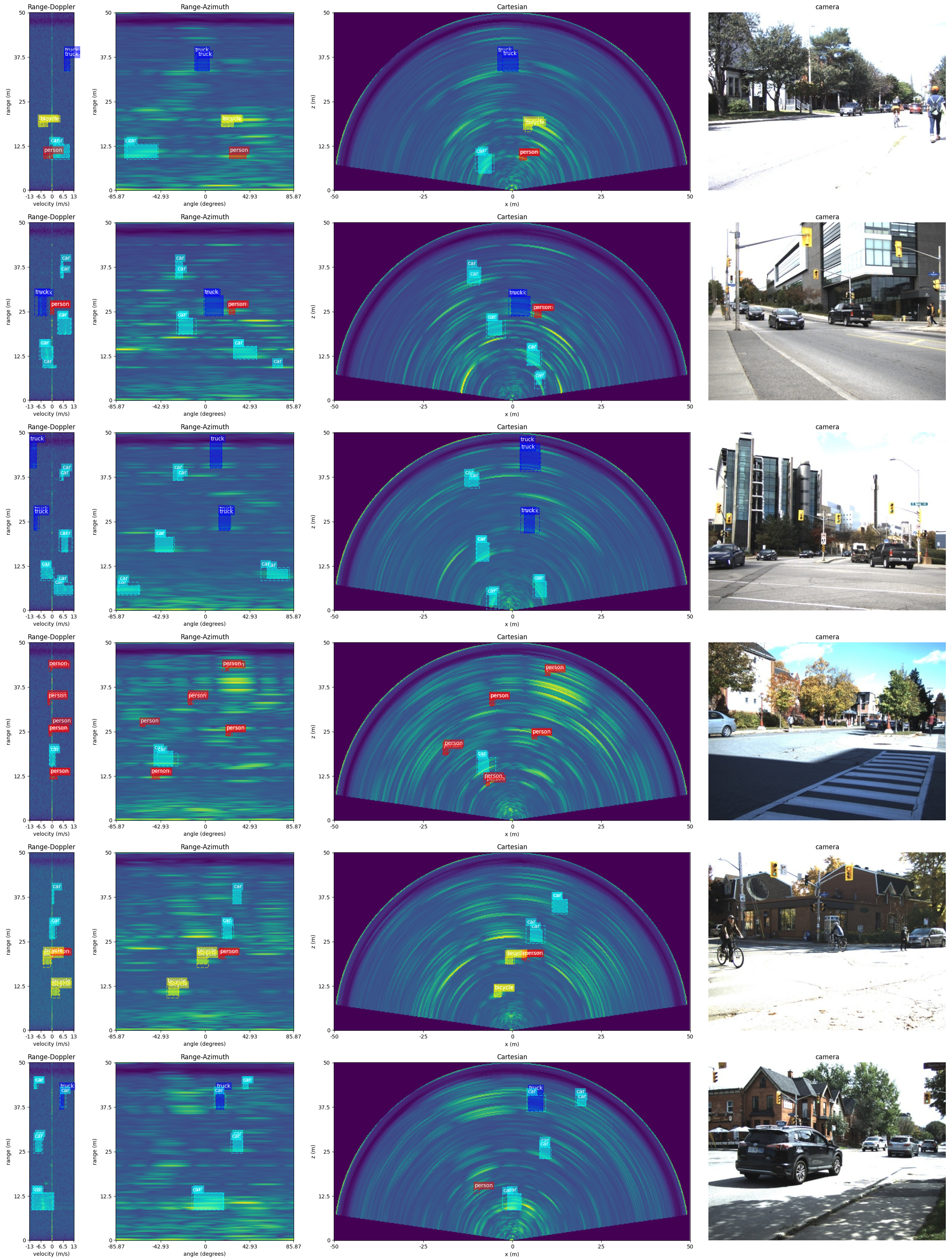
The following .gif contains inference samples from our model.
It can also be found at Youtube.
-
Our paper is accepted by 2021 18th Conference on Robots and Vision (CRV). To read the paper, see arXiv preprint or CRV Conference Version.
-
Announcement: we are still trying different backbone layers. Therefore, the current backbone layers may vary from the original implementations.
Our model is developed under
System:				Ubuntu 18.04
Python:				3.6.9
CUDA version:			10.1
TensorFlow:			>=2.3.0
For all the requirements, you can simply run
$ pip install -r requirements.txtFor those who are interested in our dataset, GoogleDrive or OneDrive.
[2021-06-05] As I have received several requests for the access of different input data types and ground truth types, I here share more data. They are available at GoogleDrive.
Please note that each folder contains entire 10158 frames, which might make it relatively difficult to download. The ADC folder contains raw radar ADC data and the gt folder contains the ground truth labels in the instance-segmentation format. The gt folder may almost reach size 1 TB, so be careful when downloading it.
[2021-07-01] Due to the reason that some people are very interested in the performance of our auto-annotation method, we uploaded two videos for the request. They are available at visual performance on ego-motion and visual performance on stationary case. More details of the auto-annotation method can be viewed in our paper.
After 1.5 months efforts with >60800 frames data capture, auto-annotation and manual correction, a stationary radar dataset for moving road users is generated. The dataset contains totally 10158 frames. Each one of them is carefully annotated, including everything that can be seen by radar but not by stereo.
For the data capture, we used the same radar configuration through the entire research. The details of the data capture is shown below.
"designed_frequency":			76.8 Hz,
"config_frequency":			77 Hz,
"range_size":				256,
"maximum_range":			50 m,
"doppler_size":				64,
"azimuth_size":				256,
"range_resolution":			0.1953125 m/bin,
"angular_resolution":			0.006135923 degrees/bin,
"velocity_resolution":			0.41968030701528203 (m/s)/bin
The dataset has totally 6 categories, different input formats and ground truth formats. All the information that stored in the dataset can be concluded as follow.
RAD:		3D-FFT radar data with size (256, 256, 64)
stereo_image:	2 rectified stereo images
gt:		ground truth with {"classes", "boxes", "cart_boxes"}
Note: for the classes, they are ["person", "bicycle", "car", "motorcycle", "bus", "truck" ].
Also Note: for the boxes, the format is [x_center, y_center, z_center, w, h, d].
Also Note: for the cart_box, the format is [x_center, y_center, w, h].
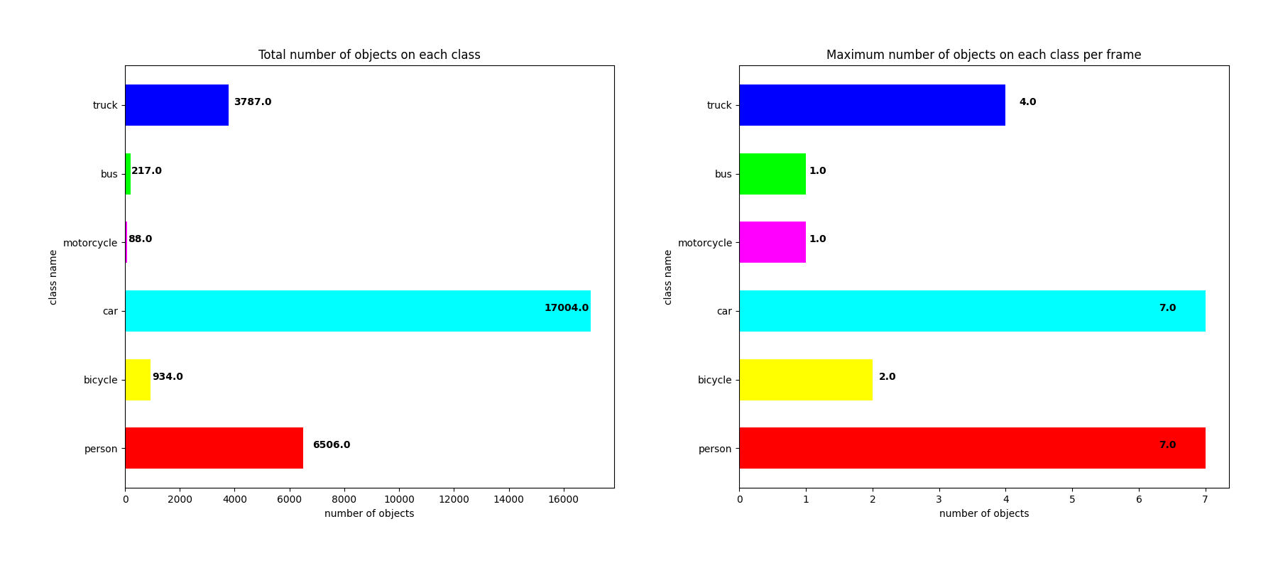
We also conducted some statistic analysis on the dataset. The figure below illustrates the number of objects of each category in the whole dataset, along with maximum number of ojbects within one single frame.
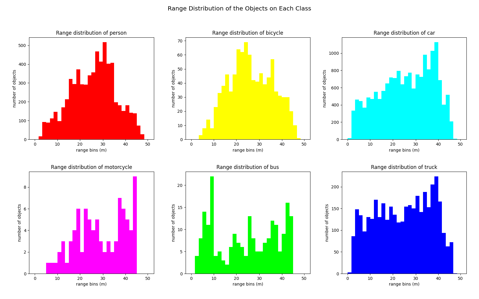
Due to the reason that most scenes are captured on either the side-walks or near the traffic lights, it appears that category "car" dominates the dataset. Still, we can see there is a good portion of the frames that have "people" inside.Since radar is mainly a distance sensor, we also did an analysis on the range distributions. The picture shown below tells about the information.
Ideally, the distribution should be Uniform. In really life scenario, it is hard to detect far-away objects (objects that almost reach the maximum range) using only 1 radar sensor. As for the objects that are too close to the radar, it becomes extremely noisy. This makes the annotation for those objects a little bit impractical.- Dataset splitting: 80% goes to trainset, and 20% goes to testset. As for the distributions of the trainset and testset, it is concluded as follow,
trainset: {'person': 5210, 'bicycle': 729, 'car': 13537, 'motorcycle': 67, 'bus': 176, 'truck': 3042}
testset:  {'person': 1280, 'bicycle': 204, 'car':  3377, 'motorcycle': 21, 'bus':  38, 'truck':  720}
Our backbone, RadarResNet, is developed based on ResNet. Details shown as below,
We also tried VGG, which is faster but lower AP.
Also shown as the image above, the RADDet has two detection heads, we call it dual detection head. These heads can detect the objects on both Range-Azimuth-Doppler (RAD) tensors and Cartesian coordinates. Both heads are developed under the inspiration of YOLOv3, YOLOv4.
Since our inputs are RAD tensors only, we propose a Coordinate Transformation block to transform the raw feature maps from Polar Coordinates to Cartesian Coordinates. The core of it is Channel-wise Fully Connected Layers.
Attention: Please keep the same directory tree as shown in GoogleDrive or OneDrive
Download the dataset and arrange it as the folloing directory tree,
|-- train
	|-- RAD
		|-- part1
			|-- ******.npy
			|-- ******.npy
		|-- part2
			|-- ******.npy
			|-- ******.npy
	|-- gt
		|-- part1
			|-- ******.pickle
			|-- ******.pickle
		|-- part2
			|-- ******.pickle
			|-- ******.pickle
	|-- stereo_image
		|-- part1
			|-- ******.jpg
			|-- ******.jpg
		|-- part2
			|-- ******.jpg
|-- ******.jpgChange the train directory in config.json as shown below,
"DATA" :
{
	"train_set_dir": "/path/to/your/train/set/directory",
	"..."
}
Also, feel free to change other training settings,
"TRAIN" :
{
	"..."
}Change the test directory in config.json as shown below,
"DATA" :
{
	"..."
	"test_set_dir": "/path/to/your/train/set/directory",
	"..."
}
Also, feel free to change other evaluate settings,
"EVALUATE" :
{
	"..."
}
Pre-trained .ckpt for RADDet is available at CheckPoint
After downloading .ckpt, create a directory ./logs and put the checkpoint file inside it.
The following figure shows the performance of our model on Test set. Last row shows the common types of false detections that found during the test.


