Copyright (c) 2019 Bart Massey
This Python 3 code demonstrates Convex Analysis using CVXPY to estimate the amplitudes of basis spectra in a noisy measured spectrum. It was written as a feasibility demo for an upcoming project.
The demo generates a random set of basis spectra. It then
simulates a measured spectrum comprised of the sum of random
proportions of the basis spectra and a uniform noise term.
CVXPY is used to estimate the spectral composition and noise
level of the measured spectrum. Finally, the results of the
simulation and analysis are displayed both textually and
graphically using matplotlib:
the analysis and figures generated are also saved as txt
and PNG files in the current directory.
Prerequisites:
- A working Python 3 installation
numpycvxpymatplotlib
It is likely that numpy and matplotlib are available in
a standard OS distro. All of the prerequisites can be
installed via pip3 install.
To run the program, you can just say python3 sd.py.
-
Each run will generate a pseudo-random number generator seed, which can be given on the command line to repeat a previous run.
-
You can set the noise level (default 0), the number of spectral samples (default 100), and the number of bases (default 5).
-
By default, the basis prevalences (amplitudes) are normalized so that the largest is between 0.5 and 1. You can also ask that the bases sum to exactly 1: a "complete" spectrum. The analysis will take this into account in its constraint model.
-
You can set the norm used for the error computation in the solver. The default is to use the L1 norm, which works pretty well: you can also choose the always popular L2 norm or the Linf norm.
-
You can choose to use only some of the bases to form the spectrum, with the rest having zero prevalence. This "sparse" spectrum could be further optimized through greedy basis pursuit — see Future Work below.
-
You can specify saving your analysis files to the current directory for later use.
Say python3 sd.py --help for program usage details.
Let's try it:
python3 sd.py --seed=27 --noise=0.2
The analysis should complete quickly and print the following text:
analysis (q=0.192, noise=0.203 (0.200)):
- olvium: 0.536 (0.453)
- afqium: 0.670 (0.674)
- emvium: 0.520 (0.504)
- ecsium: 0.134 (0.158)
- anpium: 0.138 (0.165)
Note that the basis spectra are given randomly-generated
"element names" for convenience. The numbers in parentheses
are the "true" values for which the numbers to their left
are estimates. The q is the absolute error (L1 norm) in
the approximation: it should be small.
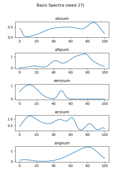
The code should also display two figures. Figure 1 shows the basis spectra chosen for the analysis.
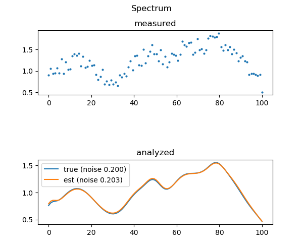
Figure 2 shows the analysis: the first graph is the simulated measurement; the second shows the true spectrum and the estimated spectrum.
The handling of the noise component still doesn't seem to be quite right. A statistician should think about it. Moving from the L2 norm to the L1 norm seemed to help here, although that may not be the right answer.
It would be useful to add a lambda parameter that disproportionately penalized the objective function for smaller basis amplitudes: this would likely improve the estimates in the case where many basis components were just not present (not a thing here).
Indeed, a parameter that outright constrained the number of basis spectra used would be helpful for some kinds of analysis. It is not clear how this would impact solver performance, however: the obvious implementation would require mixed-integer convex programming, which can be quite expensive.
A better measurement model would be a good addition, although at that point probably an analysis on real power spectral data would be even better.
Greedy basis pursuit should be used to analyze "sparse" spectra. This should give better prevalence figures in this case.
This work is made available under the "MIT License". Please
see the file LICENSE in this distribution for license
terms.

