| DC.date | DC.source | generator | title | author |
|---|---|---|---|---|
2019-10-21 |
radar\_target\_generation\_and\_detection.m |
MATLAB 9.7 |
radar\_target\_generation\_and\_detection |
Brandon Marlowe |
clear all;
clc;
%%%%%%%%%%%%%%%%%%%%%%%%%%%
% Frequency of operation = 77GHz
% Max Range = 200m
% Range Resolution = 1 m
% Max Velocity = 100 m/s
%%%%%%%%%%%%%%%%%%%%%%%%%%%
%TODO : define the target's initial position and velocity. Note : Velocity remains contant
target_range = 100;
target_velocity = 50;

radar_max_range = 200;
radar_range_resolution = 1;
radar_max_velocity = 100;
speed_of_light = 3e8;
% *%TODO* :
%Design the FMCW waveform by giving the specs of each of its parameters.
% Calculate the Bandwidth (B), Chirp Time (Tchirp) and slope (slope) of the FMCW
% chirp using the requirements above.

%Operating carrier frequency of Radar
fc = 77e9;             %carrier freq Hz
B = speed_of_light /(2 * radar_range_resolution);

% The sweep time can be computed based on the time needed for the signal to travel the unambiguous
% maximum range. In general, for an FMCW radar system, the sweep time should be at least
% 5 to 6 times the round trip time. This example uses a factor of 5.5.
t_sweep = 5.5;
t_chirp = t_sweep * 2 * (radar_max_range/speed_of_light);
slope = B / t_chirp;

%The number of chirps in one sequence. Its ideal to have 2^ value for the ease of running the FFT
%for Doppler Estimation.
Nd = 128;                   % #of doppler cells OR #of sent periods % number of chirps

%The number of samples on each chirp.
Nr = 1024;                  %for length of time OR # of range cells

% Timestamp for running the displacement scenario for every sample on each
% chirp
t = linspace(0,Nd*t_chirp,Nr*Nd); %total time for samples

%Creating the vectors for Tx, Rx and Mix based on the total samples input.
Tx = zeros(1, length(t)); %transmitted signal
Rx = zeros(1, length(t)); %received signal
Mix = zeros(1, length(t)); %beat signal


%Similar vectors for range_covered and time delay.
r_t = zeros(1, length(t));
td = zeros(1, length(t));
Running the radar scenario over the time.
for i = 1 : length(t)
  % *%TODO* :
  %For each time stamp update the Range of the Target for constant velocity.
  r_t(i) = target_range + (target_velocity*t(i));
  td(i) = (2 * r_t(i)) / speed_of_light;

  % *%TODO* :
  %For each time sample we need update the transmitted and
  %received signal.
  Tx(i) = cos(2 * pi * (fc * t(i) + 0.5 * slope * t(i)^2));
  Rx(i)  = cos(2 * pi * (fc * (t(i) - td(i)) + 0.5 * slope * (t(i) - td(i))^2));

  % *%TODO* :
  %Now by mixing the train_cellsansmit and Receive generate the beat signal
  %This is done by element wise matrix multiplication of train_cellsansmit and
  %Receiver Signal
  Mix(i) = Tx(i) .* Rx(i);
end
%TODO :
%reshape the vector into Nr*Nd array. Nr and Nd here would also define the size of
%Range and Doppler FFT respectively.
Mix = reshape(Mix, [Nr, Nd]);

% *%TODO* :
%run the FFT on the beat signal along the range bins dimension (Nr) and
%normalize.
sig_fft = fft(Mix, Nr);

% *%TODO* :
% Take the absolute value of FFT output
sig_fft = abs(sig_fft);
sig_fft = sig_fft ./ max(sig_fft); % Normalize

% *%TODO* :
% Output of FFT is double sided signal, but we are interested in only one side of the spectrum.
% Hence we throw out half of the samples.
sig_fft = sig_fft(1 : Nr/2-1);

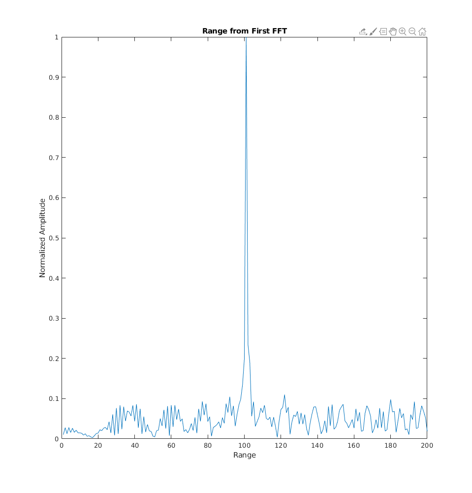
%plotting the range
%figure ('Name','Range from First FFT')

% *%TODO* :
% plot FFT output
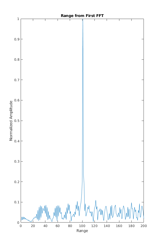
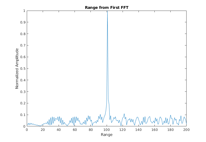
plot(sig_fft);
axis ([0 200 0 1]);
title('Range from First FFT');
ylabel('Normalized Amplitude');
xlabel('Range');
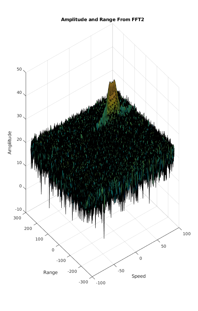
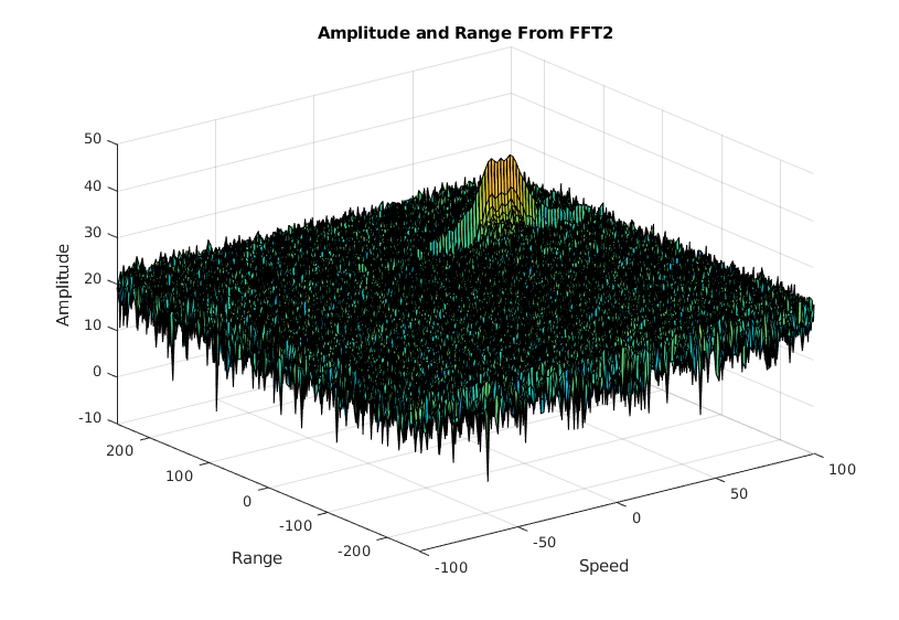
The 2D FFT implementation is already provided here. This will run a 2DFFT on the mixed signal (beat signal) output and generate a range doppler map.You will implement CFAR on the generated RDM
% Range Doppler Map Generation.

% The output of the 2D FFT is an image that has reponse in the range and
% doppler FFT bins. So, it is important to convert the axis from bin sizes
% to range and doppler based on their Max values.

Mix = reshape(Mix, [Nr, Nd]);

% 2D FFT using the FFT size for both dimensions.
sig_fft2 = fft2(Mix, Nr, Nd);

% Taking just one side of signal from Range dimension.
sig_fft2 = sig_fft2(1 : Nr/2, 1 : Nd);
sig_fft2 = fftshift(sig_fft2);

range_doppler_map = abs(sig_fft2);
range_doppler_map = 10 * log10(range_doppler_map);

%use the surf function to plot the output of 2DFFT and to show axis in both
%dimensions
doppler_axis = linspace(-100, 100, Nd);
range_axis = linspace(-200, 200, Nr/2) * ((Nr/2) / 400);

% Additional views of the surface plot
figure ('Name', 'Amplitude and Range From FFT2');
surf(doppler_axis, range_axis, range_doppler_map);
title('Amplitude and Range From FFT2');
xlabel('Speed');
ylabel('Range');
zlabel('Amplitude');
%Slide Window through the complete Range Doppler Map
% *%TODO* :
%Select the number of train_cellsaining Cells in both the dimensions.
train_cells = 10;
train_band = 8;

% *%TODO* :
%Select the number of Guard Cells in both dimensions around the Cell under
%test (CUT) for accurate estimation
guard_cells = 4;
guard_band = 4;

% *%TODO* :
% offset the threshold by SNR value in dB
offset = 1.4;

% *%TODO* :
%design a loop such that it slides the CUT across range doppler map by
%giving margins at the edges for train_cellsaining and Guard Cells.
%For every iteration sum the signal level within all the training
%cells. To sum convert the value from logarithmic to linear using db2pow
%function. Average the summed values for all of the training
%cells used. After averaging convert it back to logarithimic using pow2db.
%Further add the offset to it to determine the threshold. Next, compare the
%signal under CUT with this threshold. If the CUT level > threshold assign
%it a value of 1, else equate it to 0.


% Use RDM[x,y] as the matrix from the output of 2D FFT for implementing
% CFAR

range_doppler_map = range_doppler_map / max(range_doppler_map(:));

for row1 = train_cells + guard_cells + 1 : (Nr/2) - (train_cells + guard_cells)
  for col1 = train_band + guard_band + 1 : (Nd) - (train_band + guard_band)
    %Create a vector to store noise_level for each iteration on training cells
    noise_level = zeros(1, 1);

    for row2 = row1 - (train_cells + guard_cells) : row1 + (train_cells + guard_cells)
      for col2 = col1 - (train_band + guard_band) : col1 + (train_band + guard_band)
        if (abs(row1 - row2) > guard_cells || abs(col1 - col2) > guard_band)
          noise_level = noise_level + db2pow(range_doppler_map(row2, col2));
        end
      end
    end

    % Calculate threshold from noise average then add the offset
    threshold = pow2db(noise_level / (2 * (train_band + guard_band + 1) * 2 * (train_cells + guard_cells + 1) - (guard_cells * guard_band) - 1));
    threshold = threshold + offset;

    cell_under_test = range_doppler_map(row1,col1);

    if (cell_under_test < threshold)
      range_doppler_map(row1, col1) = 0;
    else
      range_doppler_map(row1, col1) = 1;
    end

  end
end

% *%TODO* :
% The process above will generate a thresholded block, which is smaller
%than the Range Doppler Map as the CUT cannot be located at the edges of
%matrix. Hence,few cells will not be thresholded. To keep the map size same
% set those values to 0.
range_doppler_map(range_doppler_map~=0 & range_doppler_map~=1) = 0;

% *%TODO* :
%display the CFAR output using the Surf function like we did for Range
%Doppler Response output.
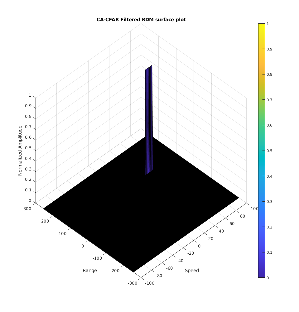
figure('Name', 'CA-CFAR Filtered RDM')
surf(doppler_axis, range_axis, range_doppler_map);
colorbar;
title( 'CA-CFAR Filtered RDM surface plot');
xlabel('Speed');
ylabel('Range');
zlabel('Normalized Amplitude');
view(315, 45);
