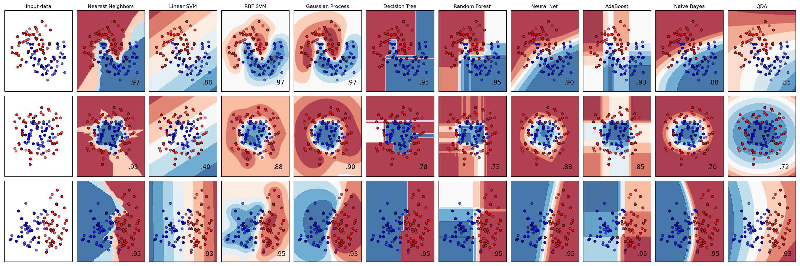
Given a set of emails, written by 2 users, objective is to classify the emails as written by one person or the other based only on the text of the email.
Acuuracy came out to be 0.97 Naive Bayes learners and classifiers can be extremely fast compared to more sophisticated methods. The decoupling of the class conditional feature distributions means that each distribution can be independently estimated as a one dimensional distribution. This in turn helps to alleviate problems stemming from the curse of dimensionality.
Particularly here, Naive bayes does work really well with Text. But with phrases which have multiple words which join to form a differrent meaning might not be best implemented by naive bayes.
training time: 127.422 s classifying time: 12.276 s Accuracy: 0.990898748578
They don't work very well when there is alot of noise in our data ie there is alot of overlap present in out datapoints. This is when Naive bayes outperform SVM. Also, it doesn't work very well in high dimenssional data as its complexity is O(n^3) with n the amount of training instances if we don't tune our parameters very well.
Effective in high dimensional spaces. Still effective in cases where number of dimensions is greater than the number of samples. Uses a subset of training points in the decision function (called support vectors), so it is also memory efficient. Versatile: different Kernel functions can be specified for the decision function. Common kernels are provided, but it is also possible to specify custom kernels.
If the number of features is much greater than the number of samples, avoid over-fitting in choosing Kernel functions and regularization term is crucial. SVMs do not directly provide probability estimates, these are calculated using an expensive five-fold cross-validation
When training an SVM with the Radial Basis Function (RBF) kernel, two parameters must be considered: C and gamma. The parameter C, common to all SVM kernels, trades off misclassification of training examples against simplicity of the decision surface. A low C makes the decision surface smooth, while a high C aims at classifying all training examples correctly. gamma defines how much influence a single training example has. The larger gamma is, the closer other examples must be to be affected.
number of features: 379 Accuracy: 0.967007963595 with significantly lower training and prediction time than number of features: 3785 Accuracy: 0.977815699659 Easy to implement and have gives us good visual interpretations. But they are prone to overfitting if we have alot of features.
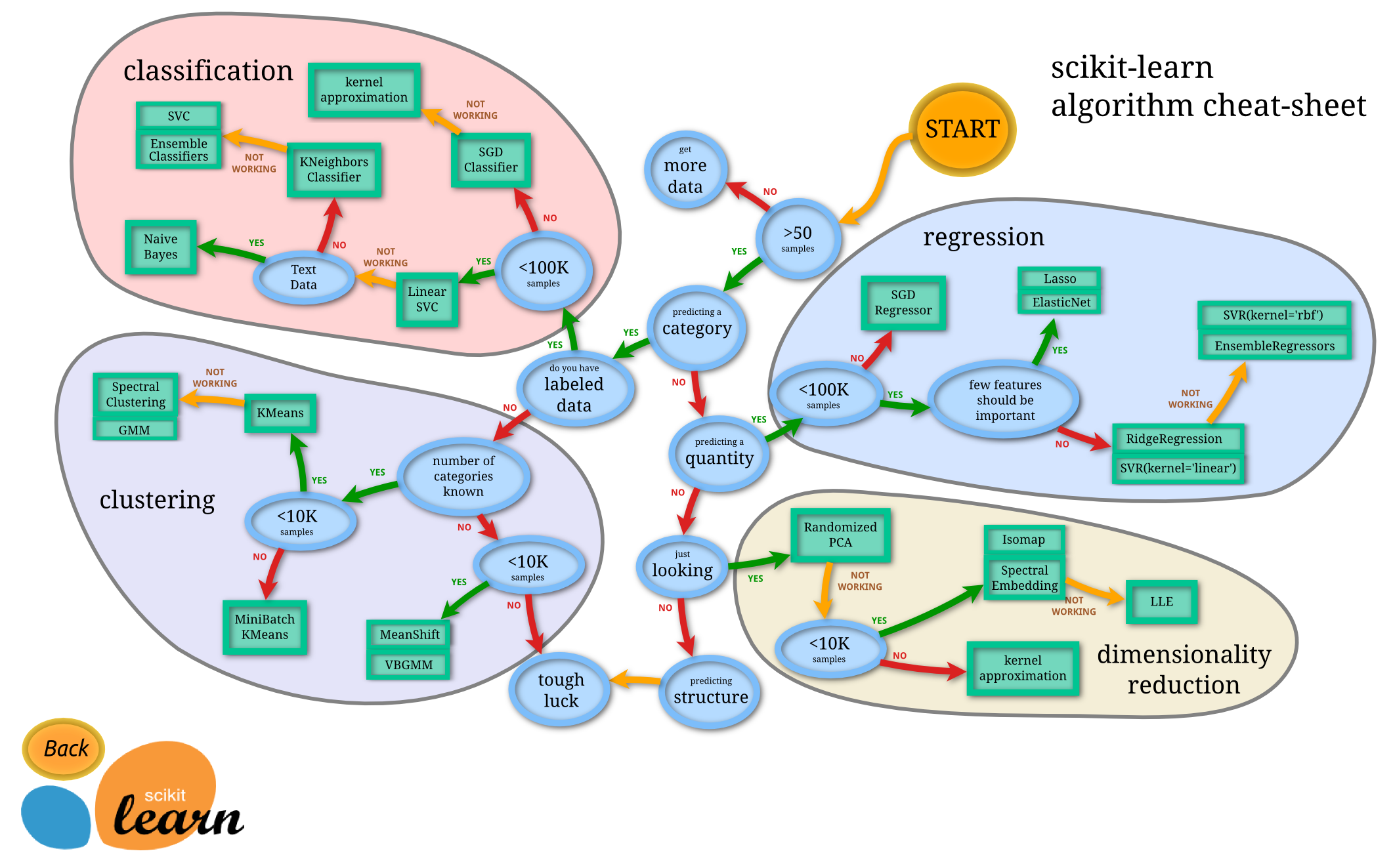
One more good resource to look what to use when could be:
Being a non-parametric method, it is often successful in classification situations where the decision boundary is very irregular. The principle behind nearest neighbor methods is to find a predefined number of training samples closest in distance to the new point, and predict the label from these. The optimal choice of the value k is highly data-dependent: in general a larger k suppresses the effects of noise, but makes the classification boundaries less distinct.
The core principle of AdaBoost is to fit a sequence of weak learners (i.e., models that are only slightly better than random guessing, such as small decision trees) on repeatedly modified versions of the data. The predictions from all of them are then combined through a weighted majority vote (or sum) to produce the final prediction. The data modifications at each so-called boosting iteration consist of applying weights w_1, w_2, …, w_N to each of the training samples. Initially, those weights are all set to w_i = 1/N, so that the first step simply trains a weak learner on the original data. For each successive iteration, the sample weights are individually modified and the learning algorithm is reapplied to the reweighted data. At a given step, those training examples that were incorrectly predicted by the boosted model induced at the previous step have their weights increased, whereas the weights are decreased for those that were predicted correctly. As iterations proceed, examples that are difficult to predict receive ever-increasing influence.
My results for Car speed classification data for Udacity "Intro to Machine Learning Course" are attached along with the repository as images.

