This is a small Julia project to do an n-body gravity simulation with command line argument processing. This is my first proper Julia project and I want to use it to learn how to use the language properly.
To use this software on your own machine, you'll have to install Julia. If you're on Windows, download the installer and tick the Add Julia to PATH box in the installer. This is necessary. If you're on MacOS or Linux, just download the binary package and put it wherever you want, just make sure you add the executable to your PATH.
To download Julia-Gravity, click the green Code button at the top of this GitHub page, and select Download ZIP. Then extract the zip file to a suitable directory.
Before first usage, open a terminal or command prompt in the directory, and run julia install_deps.jl. This will install the dependencies and will probably take some time.
Now you're ready to run gravity.jl with the arguments explained below. On MacOS and Linux, you can call it as ./gravity.jl, but on Windows, you need to call it as julia gravity.jl and then specify the arguments.
Please note: generating GIFs can take 30-60 seconds, often slower if you're trying to simulate lots of bodies or render lots of frames. This is a problem with the Julia Plots library, meaning there's very little I can do about it.
./gravity.jl [--help] -n <number> -f <frames> [-t <seconds>] [-F <filename>] [--cube] [--initial-bounds] [--quiet] [attribute options]
gravity.jl is a program designed to simulate gravity with any number of bodies and produce a GIF.
The user must specify a number of bodies with -n, and a number of frames with -f. (A value of 2000 to 4000 frames typically produces a GIF long enough to see interesting movement while being relatively quick to process, although this will vary based on other parameters.) A time step in seconds can also be optionally specified with -t. This defaults to 60 seconds.
-n and -f must be integers, but -t can be any real number.
The -F argument allows the user to optionally specify a particular filename. If not specified, a unique name will be generated. It is out.gif is available, otherwise, the names will increment like out_1.gif, out_2.gif, always using the lowest number possible. This prevents files from being overwritten.
The --cube flag will give the plot cubic bounds, making the aspect ratio less distorting, but this will likely make the action of the bodies harder to see. Leaving out the --cube flag will give the plot tight bounds, so that the camera is better focussed on the action of the bodies. This is default.
The --initial-bounds flag sets the bounds of the plot to only contain the initial positions. Normally, if one or more bodies flies far away from the initial area, then the plot will have bounds to include its final position. This means that all of the interesting motion is concentrated in the centre and is hard to see. With the --initial-bounds flag, the camera will only focus on the initial area and any bodies that fly away will be ignored. This might mean that the motion of all bodies moves out of bounds, however, and it often cuts things off on the 3 orthogonal cameras.
The --quiet flag will suppress the terminal output of the full command. It will still always be written to a file called command_log.txt along with the time the command was run, no matter what.
There are three options to specify attributes of bodies. They are as follows:
-m n,m Set the mass of body number n to be m kg.
-p n,x,y,z Set the initial position of body number n to be (x, y, z).
-v n,x,y,z Set the initial velocity of body number n to be [x, y, z].
These are all optional and if any attribute is not specified for any particular body, then it will be randomly generated with a suitable range of values for that attribute.
The program will output the full command necessary to recreate a simulation, so if you generate one with random attributes, you can use this output to generate the same simulation, but with more frames, for example. If you use the --quiet flag, the command will still be written to command_log.txt.
With the -p and -v flags, you can either specify all x,y,z coordinates or you can specify a single number in place of x,y,z to set them all to the same thing.
You can also use precise selectors, so you can specify just part of the attribute. For example, -v a,x15,z-5 will give all bodies a velocity of 15 m/s in the x direction, -5 m/s in the z direction, and a random velocity in the y direction.
Every attribute is parsed as a Float64 type, meaning that exponential notation (like 3.2e6 for 3.2 * 10^6) is allowed.
For the n in the -m and -v flags, you can use a number to specify a body like normal (the list of bodies starts at index 1), or you can use a range or group, or you can target all of the bodies with a.
A range is specified with - and is inclusive, so a range of 1-3 would target bodies 1, 2, and 3. A group is specified with . so a group of 1.4 would target bodies 1 and 4, but not 2, 3, or any other. Ranges and groups can also be combined, so, for example 1.3-5 would target bodies 1, 3, 4, and 5.
This targeting of multiple bodies in the same argument cannot be done for -p, because having multiple bodies starting in the same position doesn't make sense. The calculation of force involves dividing by distance squared, so if two bodies have the same initial position, then we'd have to divide by 0, and the program would crash.
Options are evaluated in the order that they are passed.
-v a,0 -v 1.3,10,0,0 would give all bodies a velocity of 0, except bodies 1 and 3, which would get velocities of 10 m/s in the positive x direction, and 0 m/s in the y and z directions. Order is important in this example. If we did -v 1.3,10,0,0 -v a,0 then the second flag would overwrite the first, and all bodies would get a velocity of 0.
-m a,1e20 -v a,0 would give all bodies a mass of 100 quintillion kg (a tiny mass on a planetary scale) and a velocity of 0.
./gravity.jl -n 2 -f 3000 -t 300 -m 1,6e24 -m 2,2e23 -p 1,0 -p 2,375e6,0,0 -v 1,0,0,50 -v 2,0,-250,0 would create a simulation of 2 bodies with 3000 frames and a time step of 5 minutes. Body 1 would have a mass of 6e24 kg, be located at (0, 0, 0), and have a velocity of 50 m/s in the positive z direction and 0 m/s in the x and y directions. Body 2 would have a mass of 2e23 kg, be located 375 million metres from the origin in the positive x direction, and have a velocity of 250 m/s in the negative y direction and 0 m/s in the x and z directions.
./gravity.jl -n 5 -f 5000 would create a simulation of 5 bodies with 5000 frames and a time step of 60 seconds. Every attribute of every body would be randomly generated every time this command is run, but the program will output what flags would need to be needed to generate the exact same simulation again.
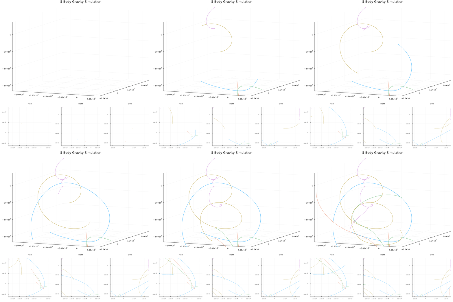
This gif was generated randomly and can be recreated with the rather verbose command ./gravity.jl -n 5 -f 2000 -t 60.0 --initial-bounds -m 1,6.3865954366971175e22 -p 1,-1.046485995157114e7,-1.1831052719693702e7,-2.6124825559583876e7 -v 1,602.2471821174969,88.0355239859146,-495.0546023282165 -m 2,3.804158913293605e22 -p 2,-4.086806858434652e6,1.9348056090842357e6,-2.8617446571503744e7 -v 2,126.54203553393488,-63.085411086555666,-1527.467404647707 -m 3,6.395369975409342e22 -p 3,6.869456059422254e6,-3.157228773415399e6,-3.161737269857981e7 -v 3,-32.53353053414486,-25.268658357766032,22.209676234563126 -m 4,4.915573852388649e23 -p 4,-2.1807002632697403e7,2.3497704125483662e7,7.232159300847966e6 -v 4,-270.2588160830812,117.2775111366177,-299.9622743423679 -m 5,1.6248795696763953e23 -p 5,-1.3716253056501677e7,8.498209911887344e6,-1.475952193047466e7 -v 5,56.02793615046529,665.5571009664108,-85.70102444687495
When a simulation is generated randomly, the corresponding command is often very long.
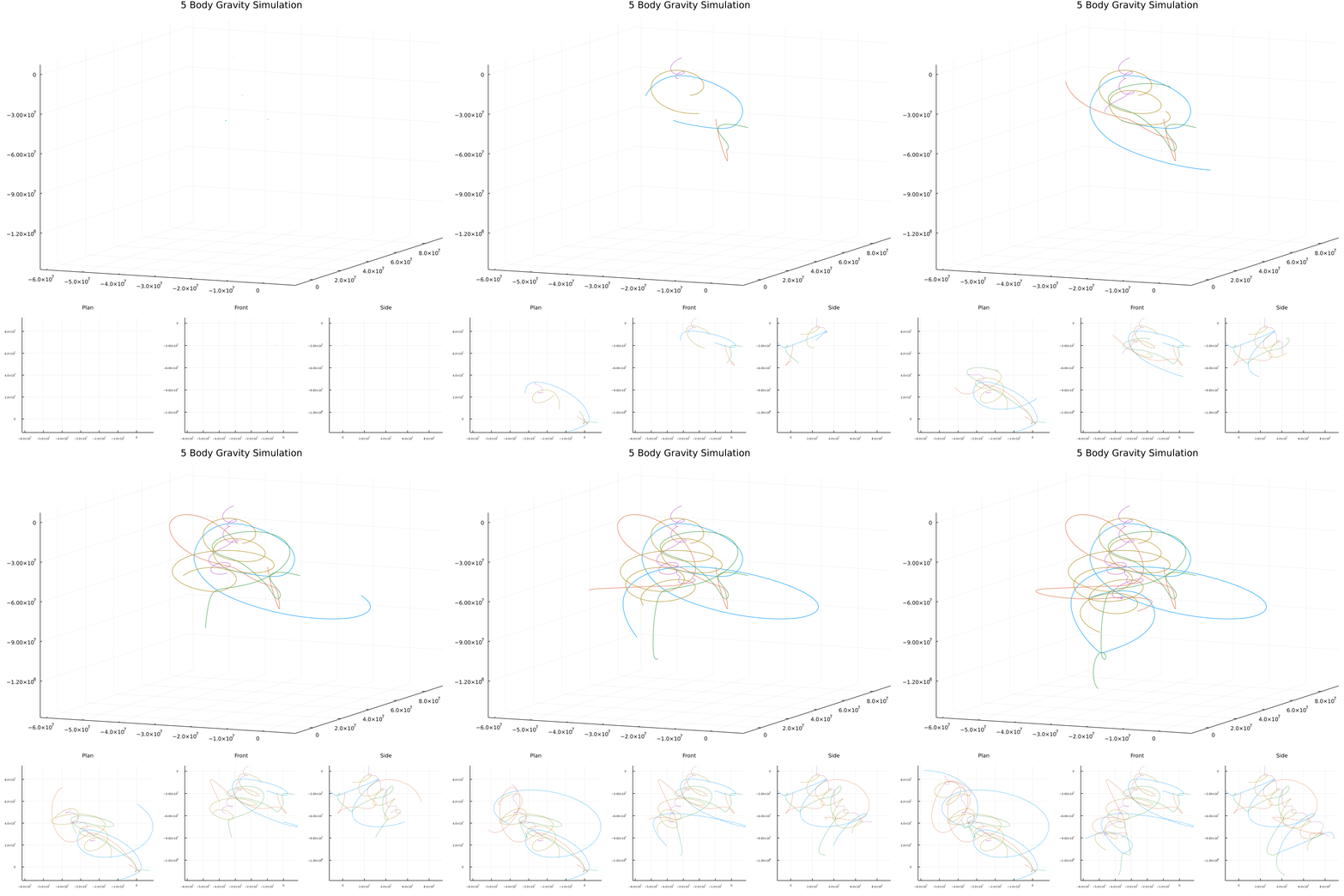
Going up to 5000 frames and removing the --initial-bounds flag shows us the more complex behaviour that's happening here:
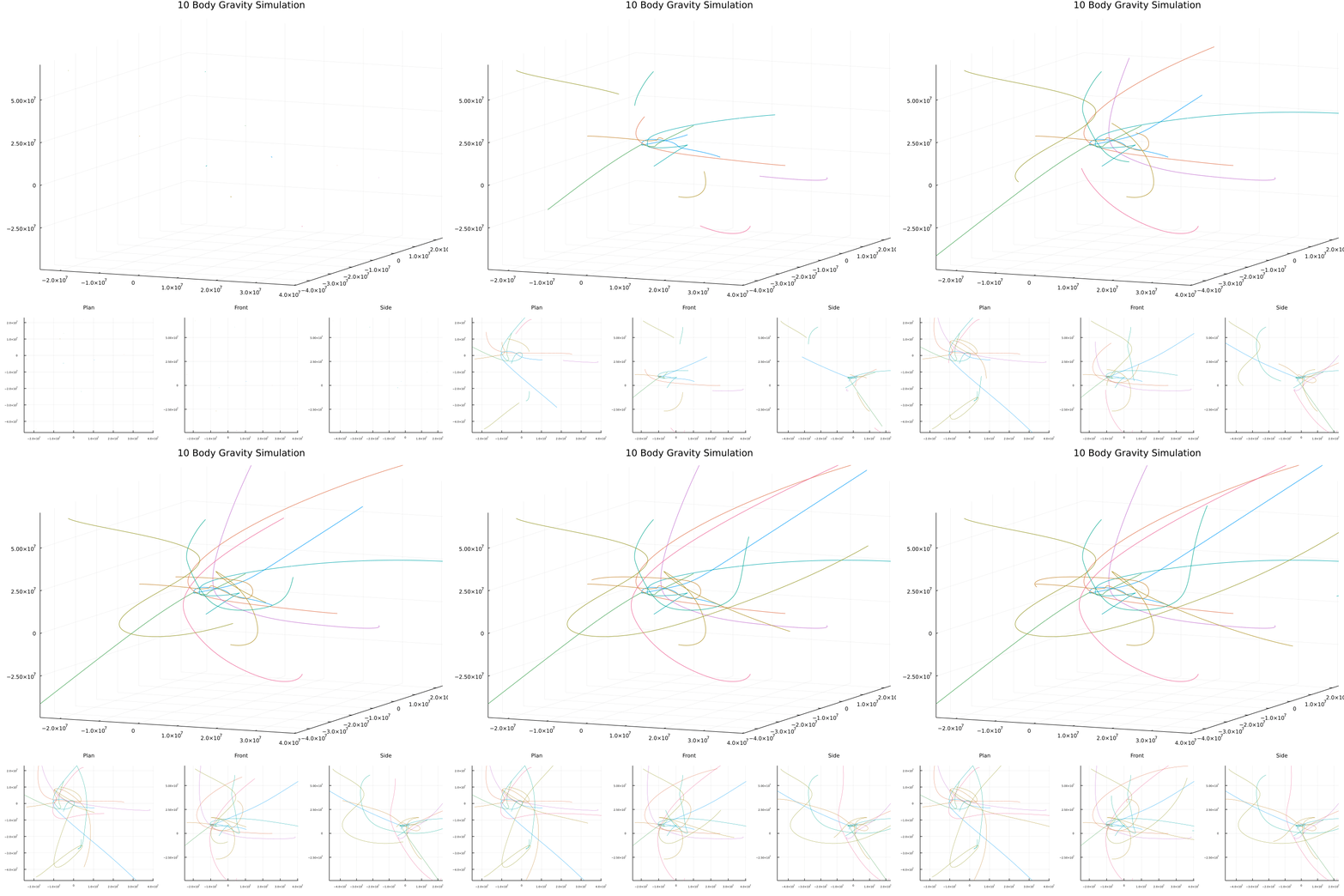
This is an example of the chaos that can ensue with a large number of bodies. This gif was generated with ./gravity.jl -n 10 -f 2000 -t 60.0 --initial-bounds -m 1,4.047467741587861e23 -p 1,1.0545281393487545e7,-2.5882862251160084e6,3.9969952578409035e6 -v 1,-492.16478021395005,-35.19123992597575,396.68555481037475 -m 2,2.2059066503628075e22 -p 2,2.543938111450544e7,633330.6076177341,4514.149223166595 -v 2,-160.7944538594973,165.27970295575054,-120.6745224031961 -m 3,2.263072682150167e23 -p 3,-4.989512826062766e6,1.3569473480153458e7,1.3868182115818229e7 -v 3,-64.91664470139949,-197.75031066397992,-158.98149998166278 -m 4,2.7283016875284848e22 -p 4,3.837887001574509e7,-3.7412746381108053e6,-3.4824621898497343e6 -v 4,187.69892322769633,-88.39890173826024,-232.95392722975305 -m 5,6.634305454886953e23 -p 5,-6.984809910588124e6,1.0081885243749723e7,-2.672612877346158e7 -v 5,582.1391040118997,-106.18887508625906,-88.09284419717028 -m 6,1.0653751225479726e23 -p 6,-5.19542659262542e6,-4.866750860307637e6,-2.6531309179450446e6 -v 6,184.6944590973707,568.3489744074186,508.346686024043 -m 7,6.570706311564152e21 -p 7,5.009794210432255e6,2.191018832360074e7,-4.6939070041895874e7 -v 7,-132.89214574033585,25.401276972145304,-772.8748727627119 -m 8,7.073129137172926e23 -p 8,-2.3739334054035924e7,-2.0408463547691586e6,1.1216348374981826e7 -v 8,284.4523287107671,-5.651649043232092,79.3085012658527 -m 9,6.2106115560258e23 -p 9,3.8308782954068636e6,-2.1716561681547455e7,6.095518400143504e7 -v 9,17.97328135423609,-427.8969282324143,-328.91586959047015 -m 10,9.76987785072852e21 -p 10,-1.894001560510119e7,-4.454985156907568e7,6.744618607127301e7 -v 10,141.12175910687577,8.8083070707169,-199.43852120397955
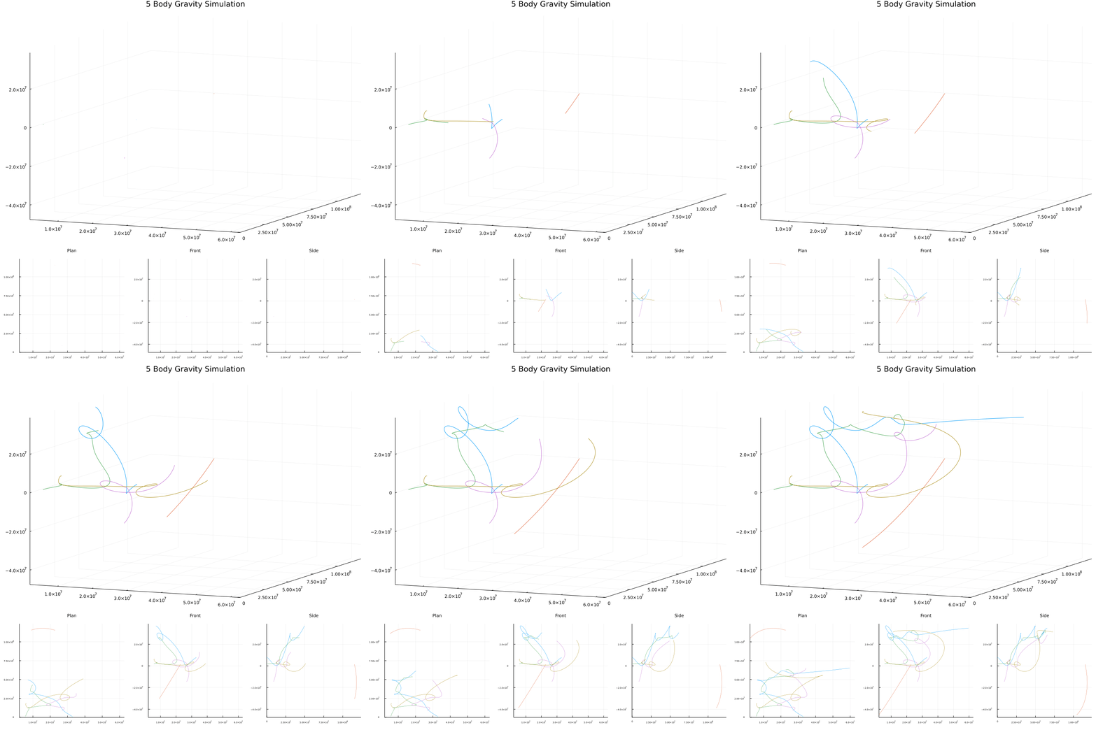
This gif is an example of the intricate and incredibly interesting behaviour that can arise from random simulations, and an example of how the orthogonal cameras help to visualise the motion of the bodies. It isn't clear with the 3D camera, but with the plan and side elevations, we can see that the orange body is really far from the other bodies, which explains its minimal gravitational interaction. This simulation can be recreated with ./gravity.jl -n 5 -f 2000 -t 60.0 -m 1,5.186220435837174e22 -p 1,3.2848406431585263e7,-258639.39262015533,7.573676103873194e6 -v 1,59.42459446412776,137.30095697714603,91.5964742068681 -m 2,2.0991132081832976e23 -p 2,2.277589000593391e7,1.1541878863163392e8,1.4438049954105443e6 -v 2,-193.60270659762398,143.53601920895767,-463.44792489260334 -m 3,2.1552661216452076e23 -p 3,5.732433698131833e6,472689.53423273424,1.9205356474706973e6 -v 3,51.16064709584796,742.8774304401079,68.53721951461738 -m 4,2.6997327815199234e23 -p 4,2.6773031514109448e7,8.904513798985038e6,-1.4546962775070718e7 -v 4,241.39073956334275,310.577374353955,644.3281196093643 -m 5,9.398564410498774e22 -p 5,6.218130764865049e6,1.7881417720981188e7,6.233510291231645e6 -v 5,-122.79099517886421,116.99239695622384,21.77927273803857


