Caution

Unfortunately, the code still doesn't work properly (needs for too low under-relaxation factors for convergence).

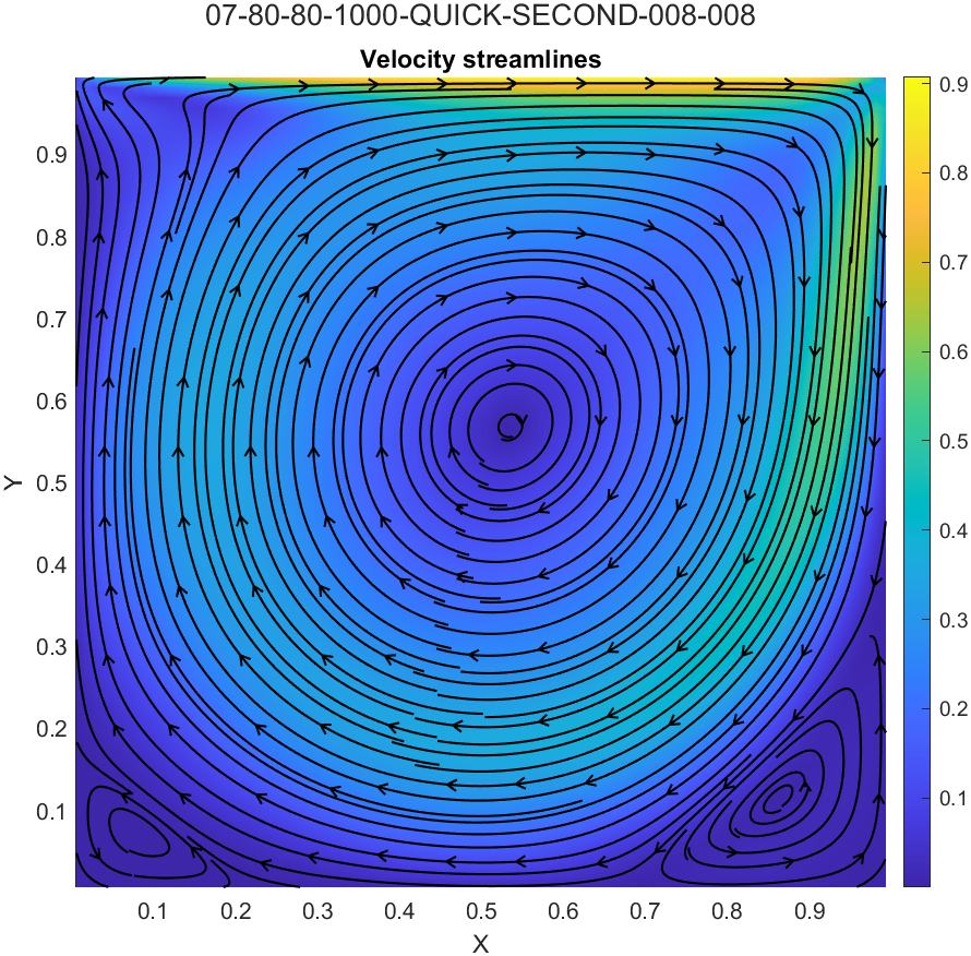
Lid-driven cavity incompressible flow (steady state)

This assignment was about solving the well known 2D lid-driven cavity incompressible flow (steady state) problem using different algorithms and schemes.

Lid-driven cavity incompressible flow solution

Problem statement

The problem consists in a square cavity with a lid moving at a constant velocity. The flow is incompressible and Reynolds number is low (Re <= 1000). Navier-Stokes equations and the pressure-velocity coupling are used to solve the problem.

Methods and schemes

The code is able to solve the problem using various methods and schemes. In particular, we can choose the following options:

Methods:
- Gauss-Siedel (SCGS)
- SIMPLE (not implemented yet)
Schemes:
- Convection schemes:
  - UDS
  - CDS
  - QUICK
  - Hybrid (not implemented yet)
- Diffusion schemes:
  - Second order central difference
  - Fourth order central difference

Data input

The code reads the input parameters from a file in JSON format.

{
    "in": {
        "uLid": 1.0,
        "geometry": {
            "x": 1.0,
            "y": 1.0
        },
        "fluid": {
            "Re": 1000
        }
    },
    "engine": {
        "mesh": {
            "nodes": {
                "Nx": 80,
                "Ny": 80
            }
        },
        "method": {
            "tolerance": 1e-05,
            "maxIter": 5000,
            "under_relaxation": {
                "u": 0.08,
                "v": 0.08
            }
        },
        "schemes": {
            "convection": "QUICK",
            "diffusion": "SECOND"
        }
    }
}

CMD input

From the command line, the possible input arguments are:

-h or --help to print the help
-v or --version to print the version
-i or --in to specify the input file path (relative or absolute). Default: -i simulations/input/input.json
-f or --format to specify the out file format. Default: -f DAT

Output

The output is saved in a DAT file and it is possible to visualize it using the MATLAB script provided in the simulations/plotting folder.

An example of the output file is:

07_80_80_1000_QUICK_SECOND_008_008
RE=1000.000000
ITERATIONS=5001
CPU_TIME=119.330000
RESIDUALS=0.000000 0.128145 0.122590 ...
VARIABLES="X", "Y", "U", "V", "P"
ZONE F=POINT, I=80, J=80
0.006250,0.006250,0.000017,-0.000021,0.044281
0.018750,0.006250,0.000113,-0.000085,0.044314
0.031250,0.006250,0.000310,-0.000123,0.044337
0.043750,0.006250,0.000558,-0.000137,0.044344
...

How to...

Clone/Download the repository

You can clone the repository either using git or downloading the zip file from the button Code on the top right of the repository.

git clone https://github.com/Bocchio01/CFD_Simulation_Engine.git

Compile the source code

Given the relavitely complexity of the code, it is recommended to use the CMake build system to compile the code. You can compile the code by typing the following command from the root folder of the repository:

mkdir build
cmake -S . -B build
cmake --build build

Run the code

If you have compiled the code using the CMake build system, you can run the code by typing the following command from the root folder of the repository:

./build/Debug/CFD_Simulation_Engine

Here is an example of how to run the code with the default parameters:

./build/Debug/CFD_Simulation_Engine -i simulations/input/input.json -f DAT

Plot the results

You can plot the results using the MATLAB script provided in the simulations/plotting folder.

Trouble shooting

If you have any trouble, please feel free to contact me.

Have a nice coding day,

Tommaso 🐼