quantstrat

Transaction-oriented infrastructure for constructing trading systems and simulation. Provides support for multi-asset class and multi-currency portfolios for backtesting and other financial research.

Overview

quantstrat provides a generic infrastructure to model and backtest signal-based quantitative strategies. It is a high-level abstraction layer (built on xts, FinancialInstrument, blotter, etc.) that allows you to build and test strategies in very few lines of code. quantstrat is still under heavy development but is being used every day on real portfolios. We encourage you to send contributions and test cases via the appropriate GitHub mediums (Pull requests and Issue tracker).

Installation

In order to install quantstrat from GitHub, you will first need to install devtools and blotter from GitHub.

install.packages("devtools") # if not installed
install.packages("FinancialInstrument") #if not installed
install.packages("PerformanceAnalytics") #if not installed

# next install blotter from GitHub
devtools::install_github("braverock/blotter")
# next install quantstrat from GitHub
devtools::install_github("braverock/quantstrat")

Example: maCross

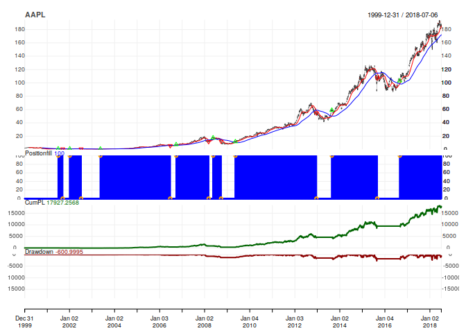
The demos in the demo folder are great for learning how to use quantstrat specifically. Below is an example of the maCross strategy, a simple moving average strategy using a short-term SMA of 50 days and a long-term SMA of 200 days.

We specify the symbol/s and currency/ies before defining the stock metadata using the stock() function from the FinancialInstrument package, available on CRAN.

stock.str='AAPL' # what are we trying it on
currency('USD')
#> [1] "USD"
stock(stock.str,currency='USD',multiplier=1)
#> [1] "AAPL"

Next we set up the rest of the backtest charateristics:

start date
initial equity
portfolio and account names
initialize Portfolio, Account and Orders objects
assign strategy object to “stratMACROSS”

startDate="1999-12-31"
initEq=1000000
portfolio.st='macross'
account.st='macross'
initPortf(portfolio.st,symbols=stock.str)
#> [1] "macross"
initAcct(account.st,portfolios=portfolio.st, initEq=initEq)
#> [1] "macross"
initOrders(portfolio=portfolio.st)
stratMACROSS<- strategy(portfolio.st)

We are now ready to add indicators, signals and rules. For more information on the theory of this approach, see below sections “About Signal-Based Strategy Modeling” and “How quantstrat Models Strategies”.

stratMACROSS <- add.indicator(strategy = stratMACROSS, name = "SMA", arguments = list(x=quote(Cl(mktdata)), n=50),label= "ma50" )
stratMACROSS <- add.indicator(strategy = stratMACROSS, name = "SMA", arguments = list(x=quote(Cl(mktdata)[,1]), n=200),label= "ma200")

stratMACROSS <- add.signal(strategy = stratMACROSS,name="sigCrossover",arguments = list(columns=c("ma50","ma200"), relationship="gte"),label="ma50.gt.ma200")
stratMACROSS <- add.signal(strategy = stratMACROSS,name="sigCrossover",arguments = list(column=c("ma50","ma200"),relationship="lt"),label="ma50.lt.ma200")

stratMACROSS <- add.rule(strategy = stratMACROSS,name='ruleSignal', arguments = list(sigcol="ma50.gt.ma200",sigval=TRUE, orderqty=100, ordertype='market', orderside='long'),type='enter')
stratMACROSS <- add.rule(strategy = stratMACROSS,name='ruleSignal', arguments = list(sigcol="ma50.lt.ma200",sigval=TRUE, orderqty='all', ordertype='market', orderside='long'),type='exit')

# if you want a long/short Stops and Reverse MA cross strategy, you would add two more rules for the short side:

# stratMACROSS <- add.rule(strategy = stratMACROSS,name='ruleSignal', arguments = list(sigcol="ma50.lt.ma200",sigval=TRUE, orderqty=-100, ordertype='market', orderside='short'),type='enter')
# stratMACROSS <- add.rule(strategy = stratMACROSS,name='ruleSignal', arguments = list(sigcol="ma50.gt.ma200",sigval=TRUE, orderqty=100, ordertype='market', orderside='short'),type='exit')

Now all we need to do is add our market data before calling the applyStrategy function to initiate the backtest.

getSymbols(stock.str,from=startDate)
#> [1] "AAPL"
for(i in stock.str)
  assign(i, adjustOHLC(get(i),use.Adjusted=TRUE))

start_t<-Sys.time()
out<-applyStrategy(strategy=stratMACROSS , portfolios=portfolio.st)
#> [1] "2001-06-27 00:00:00 AAPL 100 @ 1.443241"
#> [1] "2001-09-07 00:00:00 AAPL -100 @ 1.068518"
#> [1] "2002-01-07 00:00:00 AAPL 100 @ 1.416034"
#> [1] "2002-07-10 00:00:00 AAPL -100 @ 1.070991"
#> [1] "2003-05-16 00:00:00 AAPL 100 @ 1.162508"
#> [1] "2006-06-22 00:00:00 AAPL -100 @ 7.368322"
#> [1] "2006-09-26 00:00:00 AAPL 100 @ 9.598111"
#> [1] "2008-03-07 00:00:00 AAPL -100 @ 15.118788"
#> [1] "2008-05-19 00:00:00 AAPL 100 @ 22.706005"
#> [1] "2008-09-24 00:00:00 AAPL -100 @ 15.917701"
#> [1] "2009-05-14 00:00:00 AAPL 100 @ 15.205353"
#> [1] "2012-12-11 00:00:00 AAPL -100 @ 67.548859"
#> [1] "2013-09-11 00:00:00 AAPL 100 @ 59.474586"
#> [1] "2015-08-31 00:00:00 AAPL -100 @ 104.390999"
#> [1] "2016-08-31 00:00:00 AAPL 100 @ 100.325439"
#> [1] "2018-12-24 00:00:00 AAPL -100 @ 143.924454"
#> [1] "2019-05-07 00:00:00 AAPL 100 @ 199.698502"
end_t<-Sys.time()
print(end_t-start_t)
#> Time difference of 0.1832633 secs

Before we can review results using chart.Posn(), we update the portfolio.

start_t<-Sys.time()
updatePortf(Portfolio='macross',Dates=paste('::',as.Date(Sys.time()),sep=''))
#> [1] "macross"
end_t<-Sys.time()
print("trade blotter portfolio update:")
#> [1] "trade blotter portfolio update:"
print(end_t-start_t)
#> Time difference of 0.03264308 secs

chart.Posn(Portfolio='macross',Symbol=stock.str, TA=c("add_SMA(n=50,col='red')","add_SMA(n=200,col='blue')"))

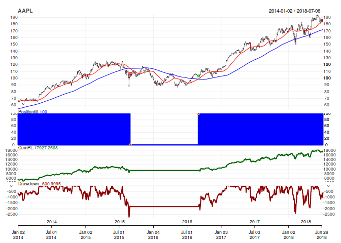
If you would like to zoom into a particular period, you can use quantmod’s zoomChart().

quantmod::zoomChart()

zoom_Chart('2014::2018')

Warning

A backtest cannot be unseen. In the words of Lopez de Prado from his book Advances in Financial Machine Learning, “Backtesting is one of the most essential, and yet least understood, techniques in the quant arsenal. A common misunderstanding is to think of backtesting as a research tool. Researching and backtesting is like drinking and driving. Do not research under the influence of a backtest. …A good backtest can be extremely helpful, but backtesting well is extremely hard.”

For a comprehensive overview of an hypothesis based approach to research and backtesting, see Developing & Backtesting Systematic Trading Strategies.

Resources

Below is a growing list of resources (some actively being developed) as relates to quantstrat:

The demo scripts in the demo folder
Datacamp course presented by quantstrat contributor Ilya Kipnis covering the basics of strategy development using quantstrat and R.
2018 R/Finance quantstrat seminar workshop presented at R/Finance 2018. The markdown source for this workshop is included with quantstrat in the vignettes directory.
Backtesting Strategies with R by Tim Trice
Guy Yollin presentations
2013 presentation by quantstrat authors Jan Humme and Brian Peterson

About Signal-Based Strategy Modeling

A signal-based strategy model first generates indicators. Indicators are quantitative values derived from market data (e.g. moving averages, RSI, volatility bands, channels, momentum, etc.). Indicators should be applied to market data in a vectorized (for fast backtesting) or streaming (for live execution) fashion, and are assumed to be path-independent (i.e. they do not depend on account / portfolio characteristics, current positions, or trades).

The interaction between indicators and market data are used to generate signals (e.g. crossovers, thresholds, multiples, etc.). These signals are points in time at which you may want to take some action, even though you may not be able to. Like indicators, signals may be applied in a vectorized or streaming fashion, and are assumed to be path-independent.

Rules use market data, indicators, signals, and current account / portfolio characteristics to generate orders. Notice that rules about position sizing, fill simulation, order generation / management, etc. are separate from the indicator and signal generation process. Unlike indicators and signals, rules are generally evaluated in a path-dependent fashion (path-independent rules are supported but are rare in real life) and are aware of all prior market data and current positions at the time of evaluation. Rules may either generate new or modify existing orders (e.g. risk management, fill, rebalance, entry, exit).

How quantstrat Models Strategies

quantstrat uses FinancialInstrument to specify instruments (including their currencies) and uses blotter to keep track of transactions, valuations, and P&L across portfolios and accounts.

Indicators are often standard technical analysis functions like those found in TTR; and signals are often specified by the quantstrat sig* functions (i.e. sigComparison, sigCrossover, sigFormula, sigPeak, sigThreshold). Rules are typically specified with the quantstrat ruleSignal function.

The functions used to specify indicators, signals, and rules are not limited to those mentioned previously. The name parameter to add.indicator, add.signal, and add.rule can be any R function. Because the supporting toolchain is built using xts objects, custom functions will integrate most easily if they return xts objects.

The strategy model is created in layers and makes use of delayed execution. This means strategies can be applied–unmodified–to several different portfolios. Before execution, quantstrat strategy objects do not know what instruments they will be applied to or what parameters will be passed to them.

For example, indicator parameters such as moving average periods or thresholds are likely to affect strategy performance. Default values for parameters may (optionally) be set in the strategy object, or set at call-time via the parameters argument of applyStrategy (parameters is a named list, used like the arguments lists).

quantstrat models orders, which may or may not become transactions. This provides a lot of extra ability to evaluate how the strategy is actually working, not working, or could be improved. For example, the performance of strategies are often affected by how often resting limit orders are changed / replaced / canceled. An order book allows the quantitative strategist to examine market conditions at the time these decisions are made. Also, the order history allows for easy computation of things that are important for many strategies, like order-to-fill ratios.

Contributing

Please see the contributing guide.

Bojan-Tomic/quantstrat