Design the following types of RF pulses:
Singleband pulses with the options:
- Linear-phase, minimum-phase, quadratic-phase
- Excitation, refocusing and matched-excitation refocusing
- Using Least-squares or CVX optimization
Multiband pulses:
- Phase-optimized (Wong ISMRM 2012)
- Time-shifted (Auerbach MRM 2013)
- Root-flipped (Sharma MRM 2015)
- VERSE-Multiband (Our work in Abo Seada MRM 2018)
- VERSE-Multiband with GIRF correction (Abo Seada ISMRM 2017)
- PINS (Norris MRM 2011)
- Multi-PINS (Eicher MRM 2014)
This code relies on the following repos:
- AM_multiband (https://github.com/mriphysics/AM_multiband)
- verse-mb (https://github.com/mriphysics/verse-mb)
Both have already been incorporated in this repo, for convenience. At the time of writing they are exact copies.
PINS and Multi-PINS code has been further developed from Will Grissoms' repo: (https://bitbucket.org/wgrissom/lowpeakpowermbrf).
Also relies on
- CVX from (http://cvxr.com/cvx/).
- Pauly's RF tools from (http://rsl.stanford.edu/research/software.html).
Open the script dz_multiband_example.m - all the variables which will affect your pulse design are in the top section.
First decide if you want to base your design on a existing RF pulse, or design a new RF pulse subject to your application.
% Basic configurations - Load or design a new base SB pulse?
Nt = 2048; %<-- set number of time-points
gamma_mT = 2*pi*4.257*1e4; %<--- same as in minTime gradient function
load_SB_pulse = 1;  %<-- set to 1 to use precalculated Single-band pulse
flip = 180*pi/180; %<-- set flip-angle.
If load_SB_pulse is 1, I have some tb2-10 refocusing pulses stored in
SB_SLR_cvxdesign_flip180_quad_Mar27. If you have access to vendor RF pulses, they can be
loaded in the same way - but you must specify the time-bandwidth product manually.
Then set mb_type to one of the multiband type pulses, the number of slices, time-bandwidth product (integer from 2-10), and slice separation.
%<-- Set what type of multiband pulse. Choose from
%    'no' : Non-optimized [Larkman 1991]
%    'po' : Phase-optimized [Hennig 1992, Wong 2013, Malik 2014]
%    'ts' : Time-shifting [ Auerbach MRM 2013]
%    'rf' : Root-flipping [Sharma MRM 2015]
%          The following four methods are described in Abo Seada MRM 2018
%    'mbv': Multiband (po) pulse followed by VERSE
%    'vmb': VERSE followed by multiband (Better for gradients!).
%    'mbvg' : Multiband VERSE pulse with GIRF-correction
%    'vmbg' : VERSE-multiband pulse with GIRF-correction (recommended..!)
%    'pins' : PINS pulses (Norris 2011)
%    'multipins' : MultiPINS pulses (Eichner 2014)

mb_type = 'no';
mb = 4; %<-- Number of slices (Multiband factor)
tb = 6; %<-- Time-bandwidth product.
bs = 10;%<-- band separation (in units of slice-thicknesses)
slthick = 2*1e-3; %<-- slice thickness [mm]
gradientslopes = 1; %<-- Set to 1 for sloping gradients at start and end.
Finally, there are some hardware parameters you can use. In this case the b1max is the most significant one as it
sets the peak B1 amplitude, and thus the RF pulse duration.
maxb1 = 13*1e-3; % <--- peak B1 [mT]
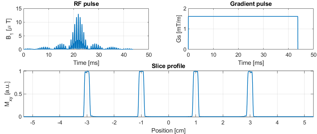
The result should look like this

My top pick for a MB spin-echo difussion sequence!
First design a new RF pulse. Set load_SB_pulse to 0, and you can use the singleband_rf function to
design a quadratic-phase pulse.
Find this bit of code in the top section:
    % Example 2: Design a new pulse using the dz_singleband function
    Nt_dz = 256; %<-- Number of time-points used for single-band design
    d1 = 0.01;
    d2 = 0.01;

    mode = 'cvx';
    pulse_type = 'me';
    phase = 'quadratic';
    quiet=0;
    [rfsb,tb] = singleband_rf(Nt_dz,tb,flip,mode,pulse_type,phase,d1,d2,quiet);

    % Interpolate design to higher nr of time-points
    rfsb = length(rfsb)/Nt*interp1(linspace(0,1,length(rfsb)),rfsb,linspace(0,1,Nt))';
Then set mb_type to vmbg which is short for "Verse the singleband pulse, Multiband it, then Girf-correct it".
mb_type = 'vmbg';
mb = 4; %<-- Number of slices (Multiband factor)
tb = 6; %<-- Time-bandwidth product.
bs = 10;%<-- band separation (in units of slice-thicknesses)
slthick = 2*1e-3; %<-- slice thickness [mm]
gradientslopes = 1; %<-- Set to 1 for sloping gradients at start and end.
Finally, make sure you select the right GIRF depending on your system. Here, h1 corresponds to a Philips 3T system, and h2 to a Siemens 3T system.
If girf is not a structure but a 1x2 matrix, the toolbox will generate an analytical Lorentzian GIRF which looks like h1.
% % %     Select one of the three GIRFs    % % %
girf = load('h1_GIRF_20140729');disp('Using measured GIRF');
girf =load('h2_GIRF_20170901.mat');disp('Using reconstructed GIRF');
girf = [42*1e-6 42*1e-6];disp('Using analytical GIRF');
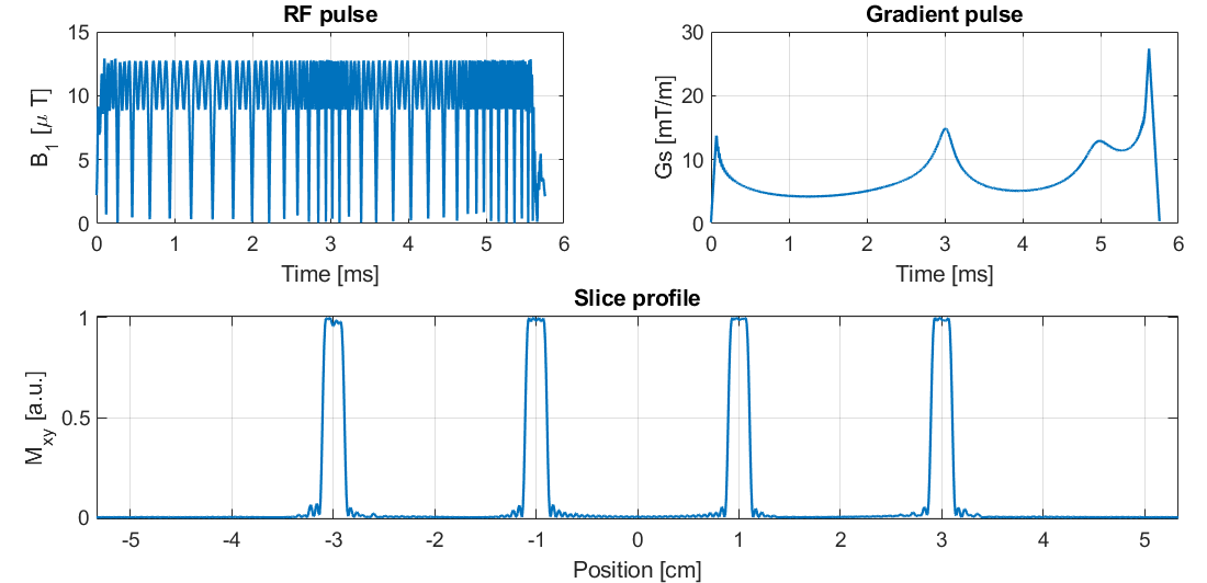
The result should look like this

Notice that the slice-profile has some errors - this is because the slice profile is simulated using the "demand" gradient.
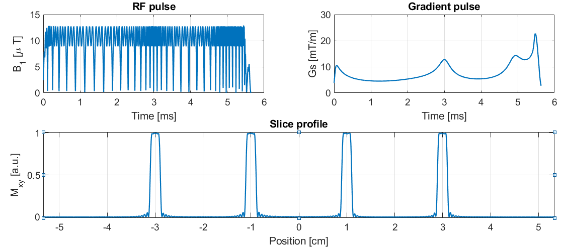
The variable return_gdem controls which of the two gradients (Demanded or GIRF-filtered) is returned.
Setting this to 0 will give the predicted slice profile, if the demand gradient is played on a scanner.
This will look like this

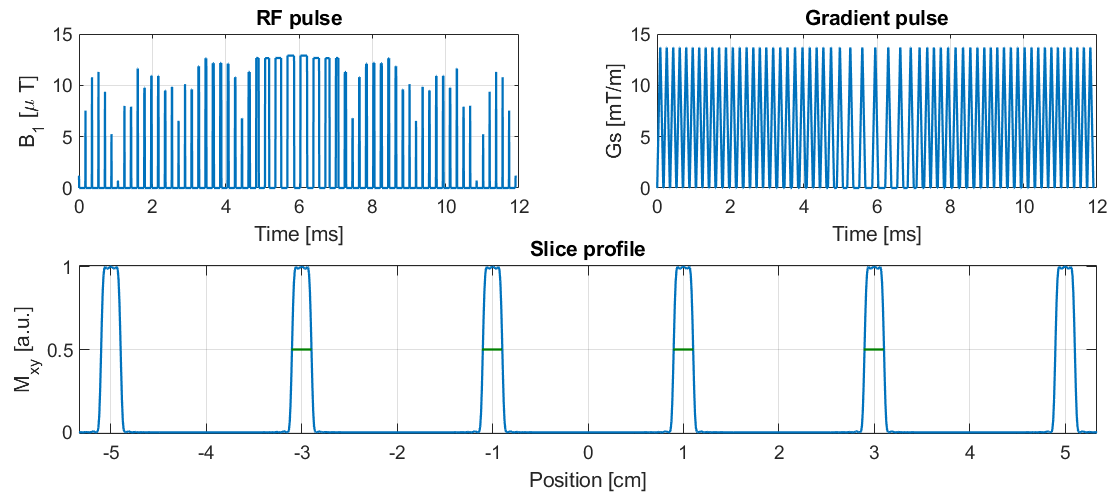
Designing a PINS pulse can easily be done by setting mb_type to 'pins'
mb_type ='pins'
load_SB_pulse = 1;  %<-- set to 1 to use precalculated Single-band pulse
The result should look like this

This section will discuss how to use the dz_single_example script.
The most common parameters you would want to change are near the top.
Nt = 256; %<-- nr of time-points
tb = 6;   %<-- Time bandwidth product

d1 = 0.01; %<-- passband ripple [%]
d2 = 0.01; %<-- stopband ripple [%]

% Set Flip angle, design mode, pulse type and phase type.
flip = pi; % Flip-angle in radians
mode = 'cvx'; % Set to cvx or ls
type = 'ref'; % Set to exc, ref or me (excitation, refocusing or matched-excitation refocusing respectively).
phase = 'linear'; % Set to linear, minimum, maximum or quadratic.
plot_fa = 0; %<-- set to 1 to plot profile in flip-angle representation
quiet = 1;  %<-- set to 1 to reduce command window output
slthick = 2*1e-3; %<-- Slice-thickness in m
These go into the singleband_rf function, and the output should look something like this
To do somehting like this, set pulse type to 'me' (short for matched-excitation) and set phase to 'quadratic'.
type = 'me'; % Set to exc, ref or me (excitation, refocusing or matched-excitation refocusing respectively).
phase = 'quadratic'; % Set to linear, minimum, maximum or quadratic.
When designing matched-excitation refocusing pulse, and a third output is requested from the singleband_rf function,
an matching excitation pulse is designed.
[rf,tb,rf_me_exc] = singleband_rf(Nt,tb,flip,mode,type,phase,d1,d2,quiet);
The easiest way to check the slice-profile of a matched-excitation pulse is the following CK representation
mxy_display = @(a180,b180)(sqrt(2)*abs(b180).^4.*sqrt(1-abs(b180).^4/2))
However, in the Bloch-simulation section there is commented where you can then simulate both excitation pulse and refocusing pulse separately. The result should be the same (as far as I checked..).
 dt90 = max(abs(rf_me_exc))/(gamma_mT*b1max);
 T90 = (length(rf_me_exc))*dt90;

 BW90 = 2*tb/T90; %<-- double BW corrects sb ripples. Why??
 Gsel90 = 2*pi*BW90/(gamma_mT*slthick)*ones(length(rf_me_exc),1);
 G90 =[0*Gsel90 0*Gsel90 Gsel90];
 % Simulate excitation pulse
 [~,~,~,~,aexc,bexc] = blochsim_CK(rf_me_exc(:)/gamma_mT/dt90,G90,pos,ones([Nz 1]),zeros([Nz 1]),'dt',dt90);
 % Simulate refocusing pulse
 [~,~,~,~,aref,bref] = blochsim_CK(rf(:)/gamma_mT/dt,G,pos,ones([Nz 1]),zeros([Nz 1]),'dt',dt);

 % This is the product of an CK excitation profile 2*alpha*beta and refocusing profile beta^2.
 mxy = 2*conj(aexc(:,end)).*bexc(:,end).*bref(:,end).^2;