This is the code for our paper Uncovering the Topology of Time-Varying fMRI Data using Cubical Persistence, which as accepted as a spotlight for NeurIPS 2020. Please use the following temporary BibTeX when citing our paper:
@InCollection{Rieck20,
  author        = {Rieck, Bastian and Yates, Tristan and Bock, Christian and Borgwardt, Karsten and Wolf, Guy and Turk-Browne, Nick and Krishnaswamy, Smita},
  title         = {Uncovering the Topology of Time-Varying {fMRI} Data using Cubical Persistence},
  year          = {2020},
  eprint        = {2006.07882},
  archiveprefix = {arXiv},
  primaryclass  = {q-bio.NC},
  pubstate      = {forthcoming},
  booktitle     = {Advances in Neural Information Processing Systems~33~(NeurIPS)},
  publisher     = {Curran Associates, Inc.},
}
You will find numerous generated files such as a summary statistics and embeddings in this repository. The raw fMRI data, however, are too large to be easily re-distributed here. Please access them under https://openneuro.org/datasets/ds000228/versions/1.0.0.
The following instructions demonstrate how to use the package and how to reproduce the experiments.
The code requires poetry to be installed.
Please install this package using the suggested installation procedure
for your operating system. Afterwards, you can install the package as
follows:
poetry install
Please use poetry shell to start a shell in which the
package and its dependencies are installed. We will assume that all
commands are executed in the ephemeral code directory.
Subsequently, we will discuss how to reproduce the individual experiments and plots.
The folder results/summary_statistics contains the results of the
summary statistics calculation as JSON files. The key is the participant
id, the value is a nested dictionary with the respective time series,
calculated based on one of the summary statistics mentioned in the
paper. Calculating these summary statistics by yourself is not
possible currently because it requires the raw data. However, the file
ephemeral/scripts/calculate_summary_statistics.sh shows how to perform
this calculation provided the raw data are available.
That being said, to reproduce Figure 3a, 3b, 3c, and 3d, please run the following commands:
# For the topological summary statistics; notice that
# 'total_persistence_p1' is the same as the 1-norm we
# we used in the paper.
python embed_summary_statistics.py  -s 'total_persistence_p1' ../results/summary_statistics/brainmask.json
python embed_summary_statistics.py  -s 'infinity_norm_p1' ../results/summary_statistics/brainmask.json

# For `baseline-tt` (see comments above concerning the data):
python embed_baseline_autocorrelation.py ../results/baseline_autocorrelation/brainmask/*.npz

# For `baseline-pp` (see comments above converning the data):
python embed_baseline_autocorrelation.py ../results/baseline_autocorrelation_parcellated/brainmask/*.npz
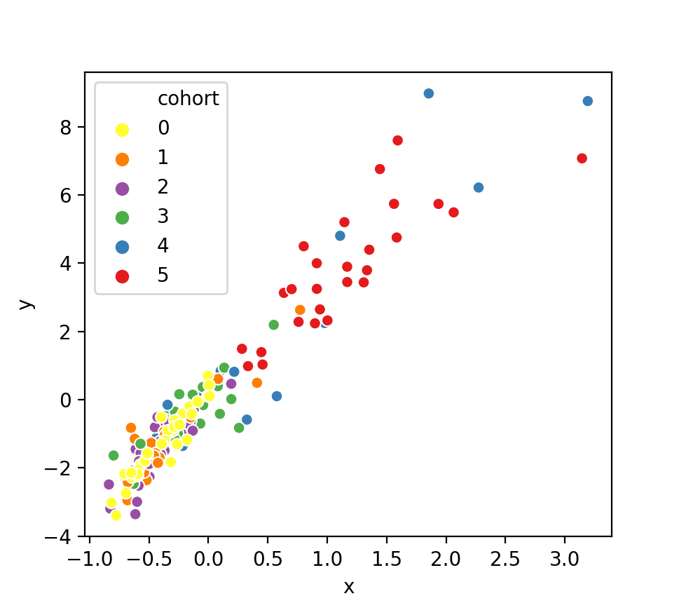
Here is an example output file (showing the infinity norm summary statistic embedding based on the whole-brain mask):
You can also calculate these embeddings for other masks, such as
occipitalmask or xormask. We have provided the necessary files
for this, but did not discuss them in the paper so far for space
reasons.
Please note that some of the plots might appear 'flipped' (with respect to the y-axis); this only affects the visualisation, but not the interpretation.
This reproduces Figure 3e in the paper.
To run the corresponding calculations, call the predict_age.py script
on different input data sets. The script is sufficiently smart to
automatically use the appropriate fitting method based on the input
data:
# For the topological summary statistics. Again, they also work for
# different brain masks (not showing all of them here). Please note
# that `total_persistence_p1` is equivalent to the `p1_norm`, as we
# describe it in the paper (the terminology in the paper was chosen
# because it is more consistent).
python predict_age.py -s 'total_persistence_p1' ../results/summary_statistics/brainmask.json
python predict_age.py -s 'infinity_norm_p1' ../results/summary_statistics/brainmask.json

# For the baseline-tt and baseline-pp experiments, respectively. For
# both experiments, other brain masks are also available.
python predict_age.py ../results/baseline_autocorrelation/brainmask/*.npz
python predict_age.py ../results/baseline_autocorrelation/occipitalmask/*.npz
python predict_age.py ../results/baseline_autocorrelation/xormask/*.npz
python predict_age.py ../results/baseline_autocorrelation_parcellated/brainmask/*.npz
python predict_age.py ../results/baseline_autocorrelation_parcellated/occipitalmask/*.npz
python predict_age.py ../results/baseline_autocorrelation_parcellated/brainmask/*.npz
Here is an example output of what you get for the infinity norm calculation:
python predict_age.py -s 'infinity_norm_p1' ../results/summary_statistics/brainmask.json

122it [00:00, 257.88it/s]
R^2: 0.37
Correlation coefficient: 0.61
MSE: 3.38
You can see the R-squared coefficient (used for fitting the model), the correlation coefficient (reported in the paper in the main text), and the mean-squared-error (reported in the supplemental materials in an extended version of the table that is shown in the main paper).
During the review period, we implemented additional baselines. To
reproduce the cells entitled tt-corr-tda and pp-corr-tda from the
table in Figure 3e, please use data from two new folders:
-
results/persistence_images_matrices: this folder contains persistence images generated from time-by-time volumes. -
results/persistence_images_from_parcellated_matrices: this folder contains persistence images generated from parcellated volumes.
The folders contain the name matrices because the persistence images
are generated from correlation matrices.
To calculate the cohort brain state trajectories shown in Figure 4, you need to use the corresponding persistence images (these files are also pre-computed because they involve the raw data). To visualise the brain state trajectories for the whole-brain mask, for example, please use the following call:
python visualise_cohort_trajectories.py -d ../results/persistence_images/brainmask_sigma1.0_r20.json
This will create a figure similar to this one:
Note that the ordering of cohorts has been swapped in the paper. As we describe in the main text, we were 'blinded' to the actual ages of the participants until the every end; hence, all visualisations are shown using the original cohort labels.
The visualisation script offers additional options, which we did not describe in the paper so far, such as a 'smoothing' process based on rolling windows. Feel free to experiment by calling
python visualise_cohort_trajectories.py --help
to see the available options! This command-line argument is understood by most of the tools that we provide, making it possible to explore the code with ease.
The corresponding cohort trajectories that we describe in the paper are
stored in the folder results/cohort_trajectories. Note that they might
be overwritten when calling the script.
To create the across-cohort-variability data (that we subsequently depict in Figure A.4 in the appendix and whose histograms are shown in Figure 4 in the main text), you can use the following code:
python analyse_variability_across_cohorts.py -d ../results/persistence_images/brainmask_sigma1.0_r20.json
This example would calculate the across-cohort variability curve of the whole-brain mask and depict it. The figure in the paper (Figure A.4 in the supplemental materials) is improved in terms of the visualisation and colour-coded according to the time, whereas the generated figure is more 'plain-looking':
Please note that the -d parameter in the script above is crucial as it
removes the first time steps (during which a blank screen is shown).
In the other scripts, this removal happens automatically, but here, we
have an option for it (it has no influence on the calculation at
other time steps, but the curve itself looks slightly different from the
ones that we report in the paper in Figure A.4). As usual, you can also
run this script for the persistences images of the other brain masks.
The corresponding curves are stored in results/across_cohort_variability.
Finally, to convert these curves into the variability histograms that we depict in Figure 4, please use the following code:
python peri_histogram_analysis.py ../results/across_cohort_variability/brainmask_sigma1.0_r20.csv
python peri_histogram_analysis.py ../results/across_cohort_variability/occipitalmask_sigma1.0_r20.csv
python peri_histogram_analysis.py ../results/across_cohort_variability/xormask_sigma1.0_20.csv
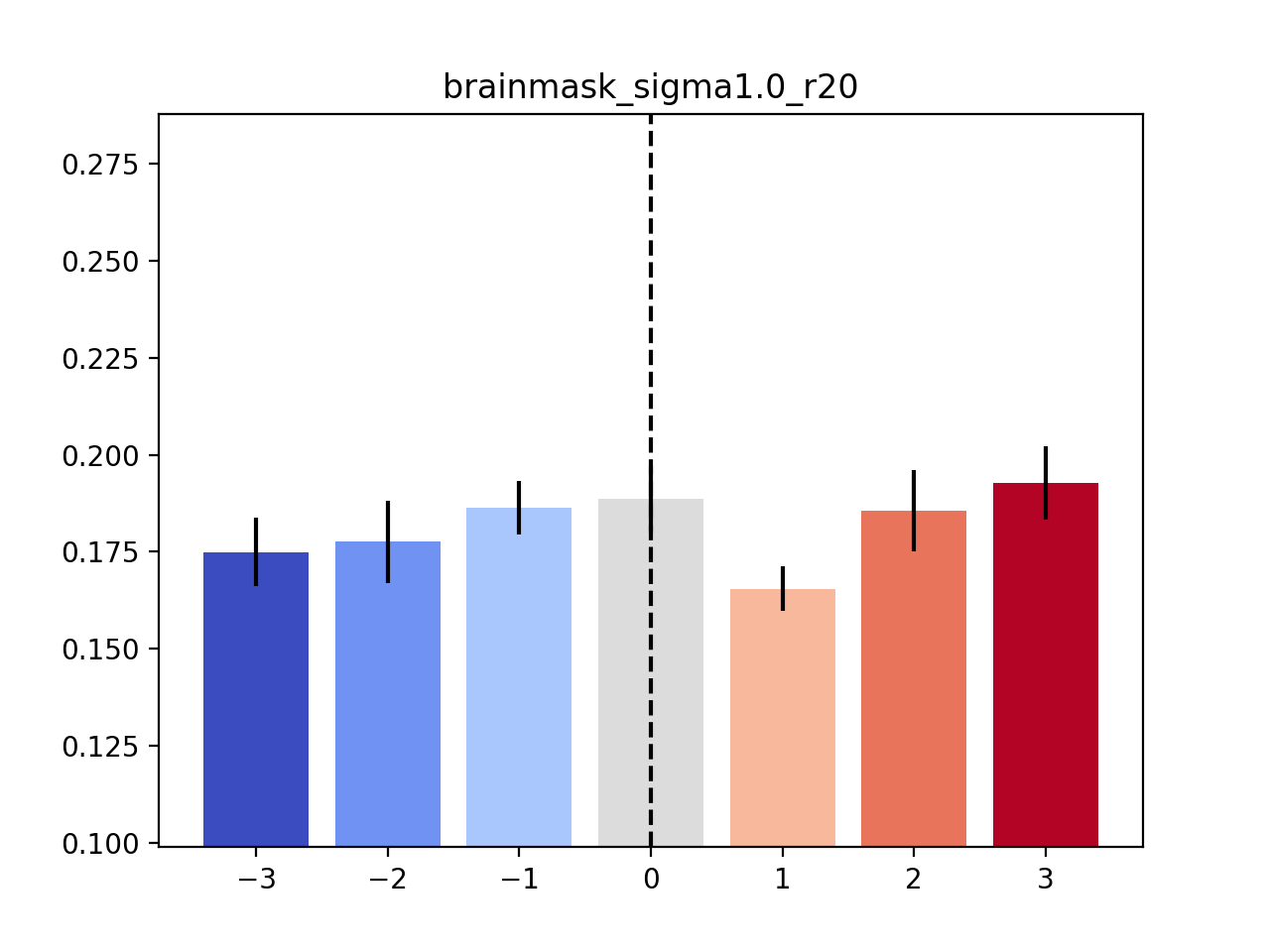
This will result in a histogram like this one (here, the whole-brain mask is used):
Finally, to show the details of the bootstrap experiments concerning the variability analysis, you can use the following code:
python peri_histogram_bootstrap_analysis.py ../results/across_cohort_variability/brainmask_sigma1.0_r20.csv
python peri_histogram_bootstrap_analysis.py ../results/across_cohort_variability/occipitalmask_sigma1.0_r20.csv
python peri_histogram_bootstrap_analysis.py ../results/across_cohort_variability/xormask_sigma1.0_20.csv
By default, this will draw 1000 bootstrap samples and visualise the corresponding histogram. Here is such a histogram (calculated based on the occipital-temporal mask), with the original value of the parameter being highlighted as a dotted vertical line:
The command-line output will show the numbers that we report in the paper. For example, the analysis based on the occipital-temporal mask will yield the following output:
python peri_histogram_bootstrap_analysis.py -b 1000 ../results/across_cohort_variability/occipitalmask_sigma1.0_r20.csv
Bootstrap: 100%|██████████████████████████████████████████████████████████████████████████████████████████████████████████████████████████████| 1000/1000 [00:15<00:00, 63.93it/s]
Theta_0: -0.0226
ASL (left) : 0.95
ASL (right): 0.04
Hence, the parameter has an achieved significance level that is significant at the 0.05 level.
The repository contains more code that we are unable to fully discuss or acknowledge in the paper because of space reasons. Please feel free to browse around; we documented most of the relevant scripts, making it possible to get a glimpse into the full pipeline.
The code pertaining to this project is released under a BSD-3-Clause License. This license does not apply to the data itself, which is released under the PDDL.


