Contains code for tackling one-dimensional quantum and two-dimensional statistical mechanics problems using tensor network algorithms. The main focus is on matrix product states (MPS) and matrix product operators (MPO), both finite and infinite.
Additionally, the framework is built upon TensorKit.jl, which provides functionality for generic symmetries.
The toolbox contains different algorithms for finding MPS representations of groundstates or leading boundary states, performing time evolution, finding excitations and much more. Check out the examples for concrete use-cases.
This package is under active development and new algorithms are added regularly. Nevertheless, the documentation is quite terse, so feel free to open an issue if you have any questions.
The package can be installed through the Julia general registry, via the package manager:
pkg> add MPSKitBecause of the heavy use of TensorKit.jl, it is recommended to install the latest version of this package as well. Additionally, several extension packages exist that provide additional symmetries, which should all be compatible with MPSKit. For example, to install the package with support for SU(N) symmetries, SUNRepresentations.jl can be used.
pkg> add TensorKitFinally, several pre-defined operators, hamiltonians and statistical mechanics models are available in MPSKitModels.jl. It is recommended to install this package too.
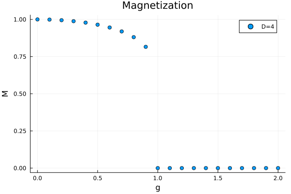
pkg> add MPSKitModelsAfter following the installation process, it should now be possible to load the packages and start simulating. For example, to obtain the groundstate of the 1D Ising model, we can use the following code:
using MPSKit, MPSKitModels, TensorKit
using ProgressMeter, Plots # for demonstration purposes

L = 16 # length of the chain
D = 4 # bonddimension
init_state = FiniteMPS(L, ℂ^2, ℂ^D)

g_values = 0:0.1:2
Z = @mpoham sum(σᶻ(){i} for i in vertices(FiniteChain(L)))

M = @showprogress map(g_values) do g
    H = periodic_boundary_conditions(transverse_field_ising(; g=g), L)
    groundstate, environment, δ = find_groundstate(init_state, H; verbose=false)
    return abs(sum(expectation_value(groundstate, Z))) / L
end

scatter(g_values, M, xlabel="g", ylabel="M", label="D=$D", title="Magnetization")
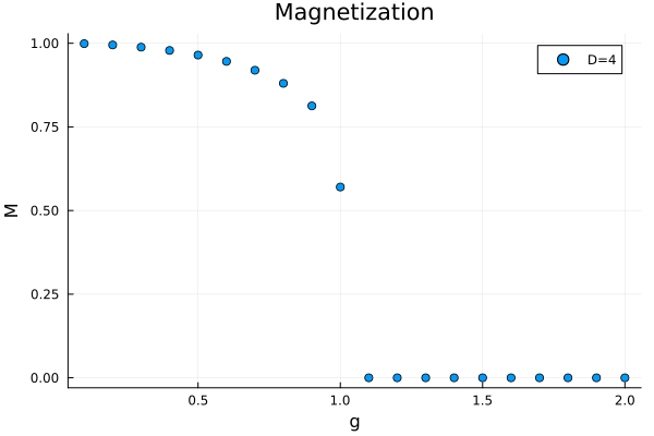
Similarly, these simulations can be carried out directly in the thermodynamic limit, with very minor code-changes:
using MPSKit, MPSKitModels, TensorKit
using ProgressMeter, Plots # for demonstration purposes

D = 4 # bonddimension
init_state = InfiniteMPS(ℂ^2, ℂ^D)

g_values = 0.1:0.1:2
Z = @mpoham sum(σᶻ(){i} for i in vertices(InfiniteChain()))

M = @showprogress map(g_values) do g
    H = transverse_field_ising(; g=g)
    groundstate, environment, δ = find_groundstate(init_state, H, VUMPS(; verbose=false))
    return abs(sum(expectation_value(groundstate, Z)))
end

scatter(g_values, M, xlabel="g", ylabel="M", label="D=$D", title="Magnetization")

