Understanding the mathematical intricacies behind machine learning models is pivotal to the whole data science process. From choosing the right model, data preparation, model tuning and evaluation, understanding how the model works is key. This repository unpacks the calculus behind stochastic gradient descent, we'll use simple linear regression as our use case.
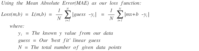
We will be using a toy data set to predict the number of calories burned given how far an athlete rode his/her bike. We will use gradient descent to perform a simple linear regression, and then benchmark our results using the least squares method.Let's begin with a refresher of the linear regression setup. The goal is to generate the line that is closest to as many data points as possible. Hence we can define our error (or loss) function to be representative of the mean distance between all data points and our line. Let’s use the Mean Absolute Error as our loss function:
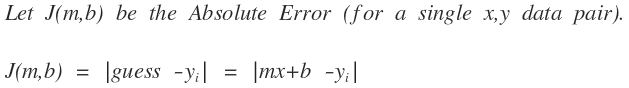
Since this is an example of Stochrastic GD and not Batch GD, so for each x,y data point pair along the way we can calculate the Absolute Error (same thing as MAE but just not averaged).
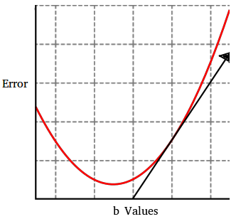
At this point, we need to find the line out of all possible lines that minimizes our loss function. Let's visualize this by graphing all possible m and b values along with their corresponding error.
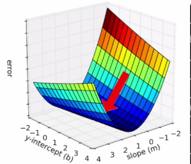
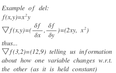
You can see that the arrow indicates our goal, but how do we get there? First we will initialize our m and b values to 0, then we will iteratively use gradient descent to change our m and b values in the direction that minimizes our loss function. The gradient is the collection of all the partial derivatives for a given multivariable function. Here is a basic usage example:
The gradient points in the direction of the greatest rate of increase of the function, and its magnitude is the slope of the graph in that direction. This is critical, for in our case if we take the gradient of our loss function then we can tell how the error changes as one of our variables change.
Let's visualize this with another example. Consider that we want to know how the error changes as b changes. The picture below is the same error surface as before, but this time let's take the partial derivative of J with regard to b (this means that m is held constant).

Now plotting error vs b in two dimensional space.
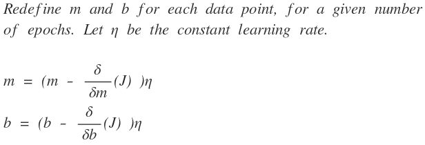
The arrow is up because the gradient points in the direction of the greatest rate of increase, yet we want to change b in the opposite direction. Thus we can redefine b to move in the opposite direction as the gradient. Note the learning rate is just a hyper-parameter that influences how quickly these changes to m and b occur.
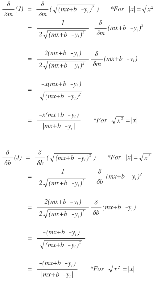
Now we can expand out our partial derivatives:
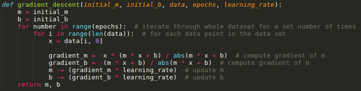
Here is the piece of code that encapsulates the whole gradient descent step.
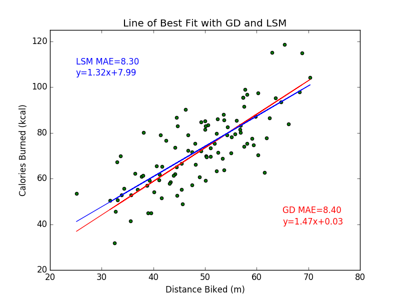
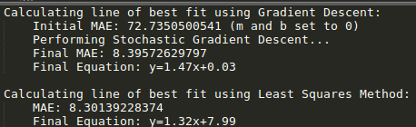
After running the code for 1000 epochs and with a learning rate of 0.0000003, we have converged to our answer. Let's also include a well known algebraic linear regression technique called the Least Squares Method (LSM) to benchmark our results.
Finally, we can visualize our results!