Jupyter Notebook Viewer
Download Powerpoint Presentation
The goal of this project was to understand the patterns of E-bike usage and create a predictive model that can forecast the number of riders per hour based on time and weather conditions.
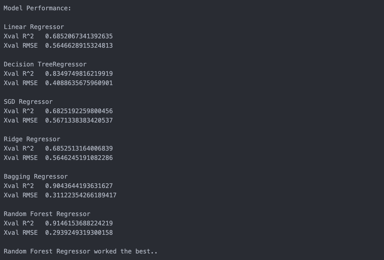
- Six models were tested: Linear Regression, Decision Tree Regressor, Random Forest Regressor, SGD Regressor, Bagging Regressor.
- Random Forest Regressor had the best performance after parameter tuning with a R^2 = 0.89 and RMSE = 0.33 (6-fold xval).
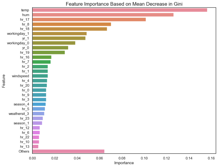
- Warmer weather, less humidity, and it being rush hour times were the best predictors of E-bike usage.
The insights from this project could enable Capital Bikeshare and similar companies to make evidence-based decisions about where and when to allocate resources, leading to increased operational efficiency and customer satisfaction.
- Increase E-Bike redistribution before rush hour to capitalize on commuter usage.
- Add E-Bike charging stations near dense employment locations.
- Offer discounts or incentives during no-optimal weather conditions.
- If E-Bike rollbacks or updates need to be done, perform them during non-peak months
The dataset is 2 years of E-bike usage, broken down by every hour of the day. All the data is publicly available from Capital Bikeshare, this includes weather data for the Washington, D.C. area.
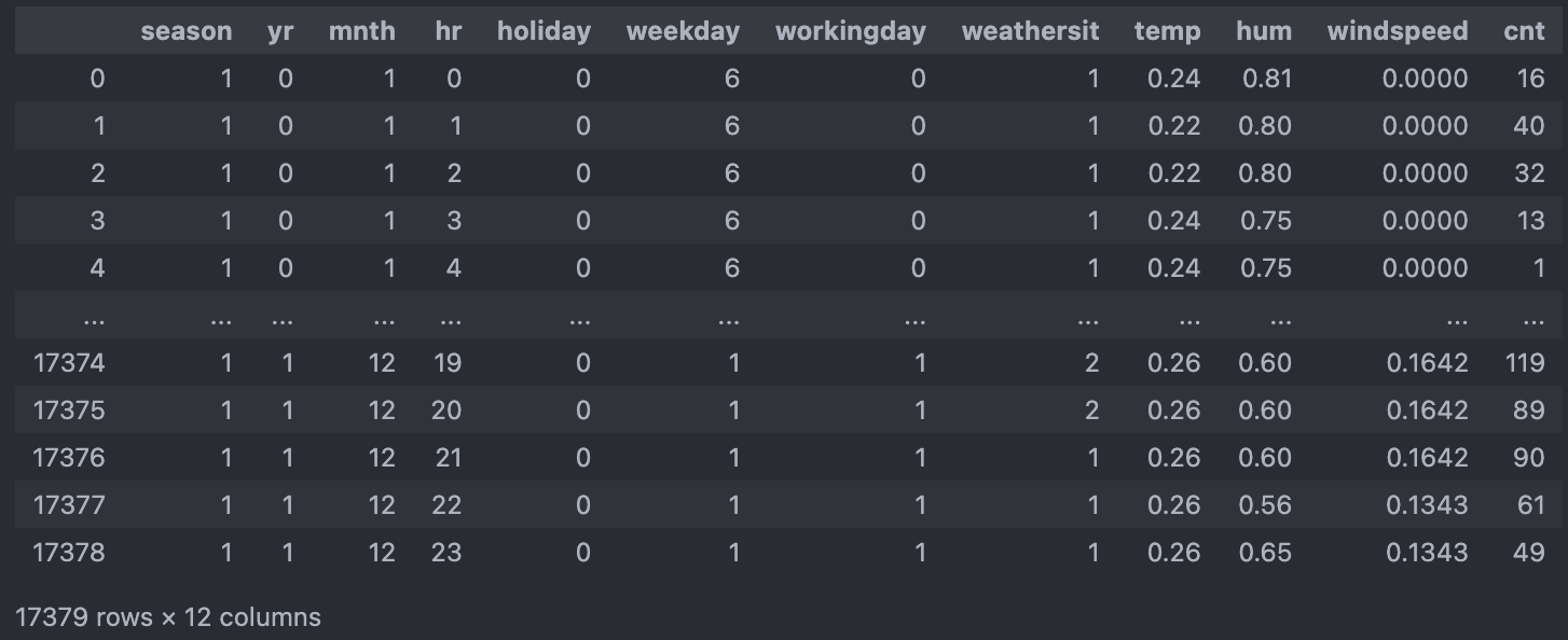
Lets take a look at all of the data in our dataset.
We have:
- 11 predictor variables
- 1 outcome variable (number of rides for that hour)
- Exploratory Data Analysis
- Checking Data Quality (data types, null values)
- Visualizing Numeric and Categorical Predictor Variables
- Explore Variables Most Correlated with E-Bike Usage
- Data Preparation
- Drop Redundant Variables
- Standard Scale Numeric Variables
- One-Hot Encode Categorical Variables
- Split Data (70 training/ 30 test)
- Model Building
- Linear Regression
- Decision Tree Regressor
- SGD Regressor
- Bagging Regressor
- Random Forest Regressor
- Compare results of R^2 and RMSE (6-fold cross-validation)
- Model Parameter Tuning
- Iterative Randomized Search for Random Forest Regressor
- Model Evaluation
- R^2, RMSE
- Residuals vs Actual, Predicted vs Actual
- Identifying the Most Important Variables, Mean Gini Decrease
- Exploratory Data Analysis
- Model Building
- Model Parameter Tuning
- Model Evaluation
- Determining Important Variables
Our categorical variables can be broken up into two types:
- Time (season, month, day, hour)
- Weather Status (Clear, Cloudy/Misty, Light Rain/Snow, Heavy Rain/Snow)
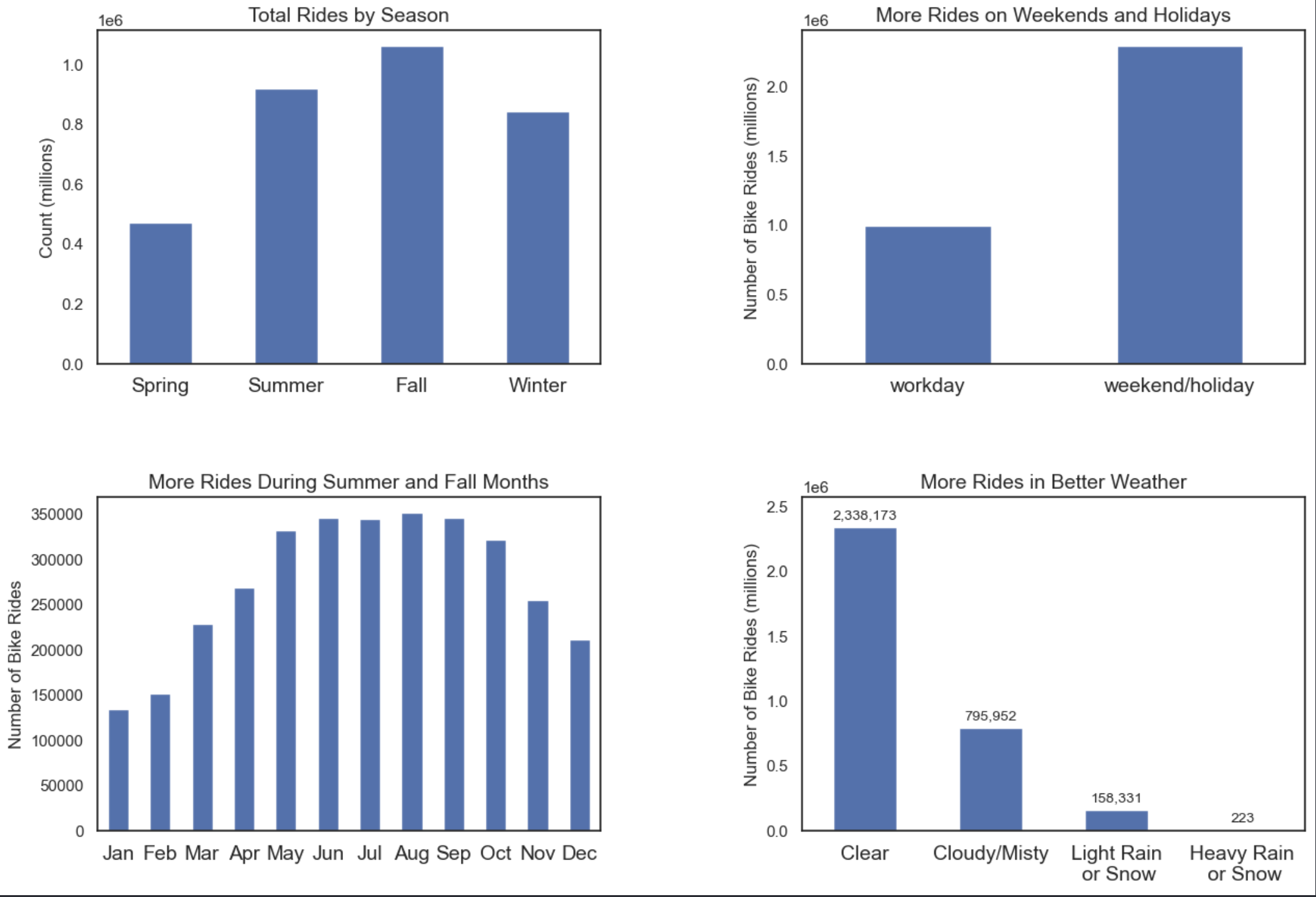
Looking at the plots there are a few takeaways:
- More rides during the summer, fall, and winter seasons (the warmer seasons)
- More rides on the weekends
- More rides when the weather is better
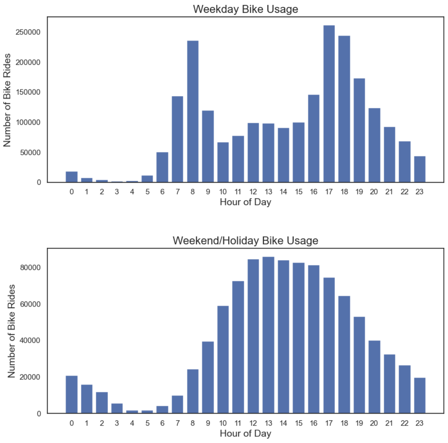
Now let's dive a little deeper and break down the average day for an E-bike user:
- Not surprisingly, rides happen most during the waking hours of a day
- Peak usage times happen during work days when people commute to and from work
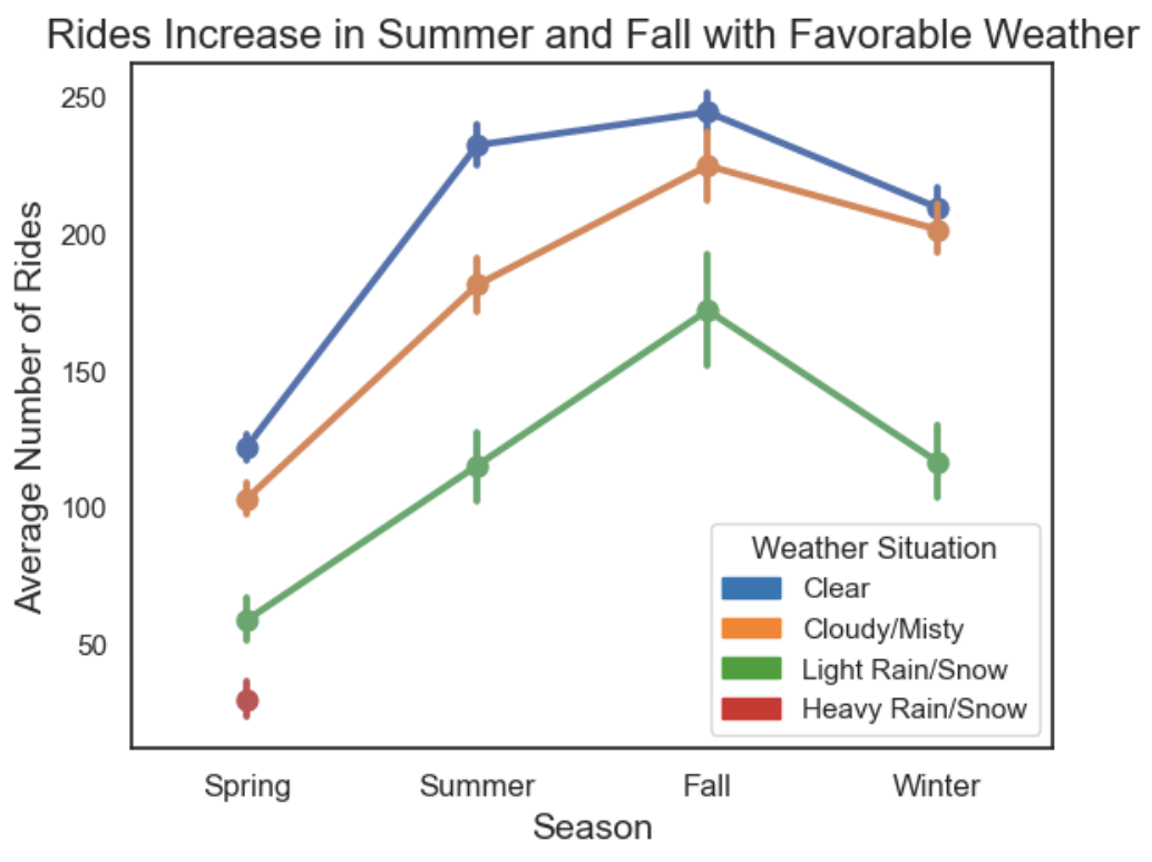
Finally let's break down the interplay between weather for a given season:
- Bad weather really does dissuade riders, regardless of season
- Again we see a trend for more rides during warmer months
Explanation of Weather Situations:
- Clear: Clear, Few clouds, Partly cloudy, Partly cloud
- Cloudy/Misty: Mist or Cloudy, Mist or Broken clouds, Mist or Few clouds, Mist
- Light Rain/Snow: Light Snow, Light Rain or Thunderstorm or Scattered clouds, Light Rain or Scattered clouds
- Heavy Rain/Snow: Heavy Rain or Ice Pallets or Thunderstorm or Mist, Snow or Fog
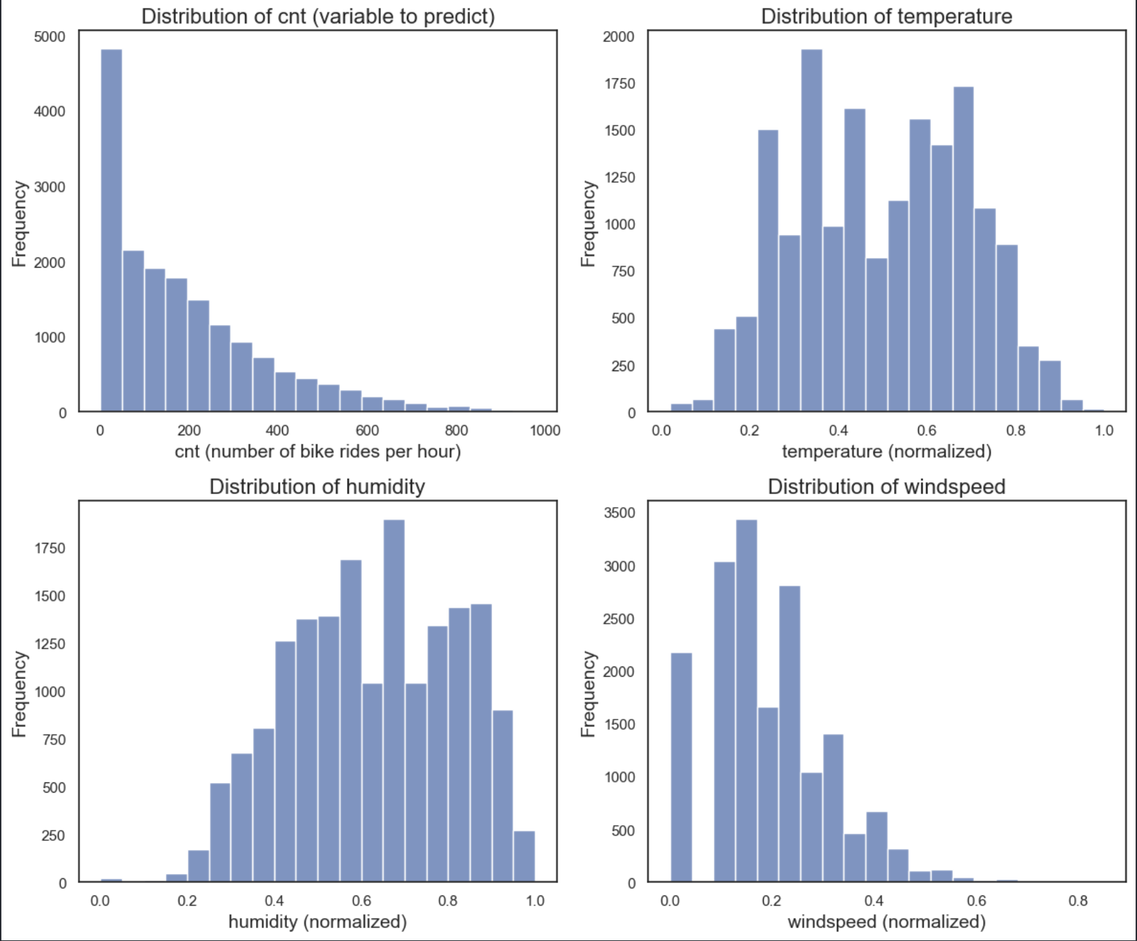
Our categorical variables are the following:
- Temperature
- Humidity
- Wind speed
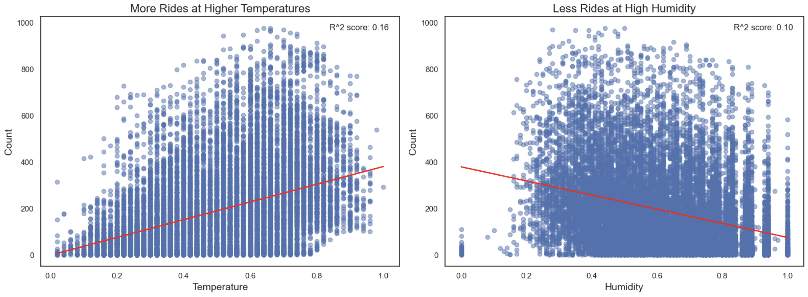
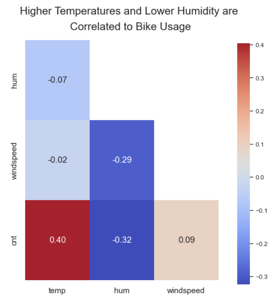
Creating a quick Pearson's Correlation heatmap we can see:
- More rides in higher temperatures
- Less rides in higher humidities
- Rides are pretty indifferent about weather it's windy out
In order to train our models, the data was split into 70% training/ 30% testing
From this point on in the analysis, we will focus on the top performing model: Random Forests Regressor
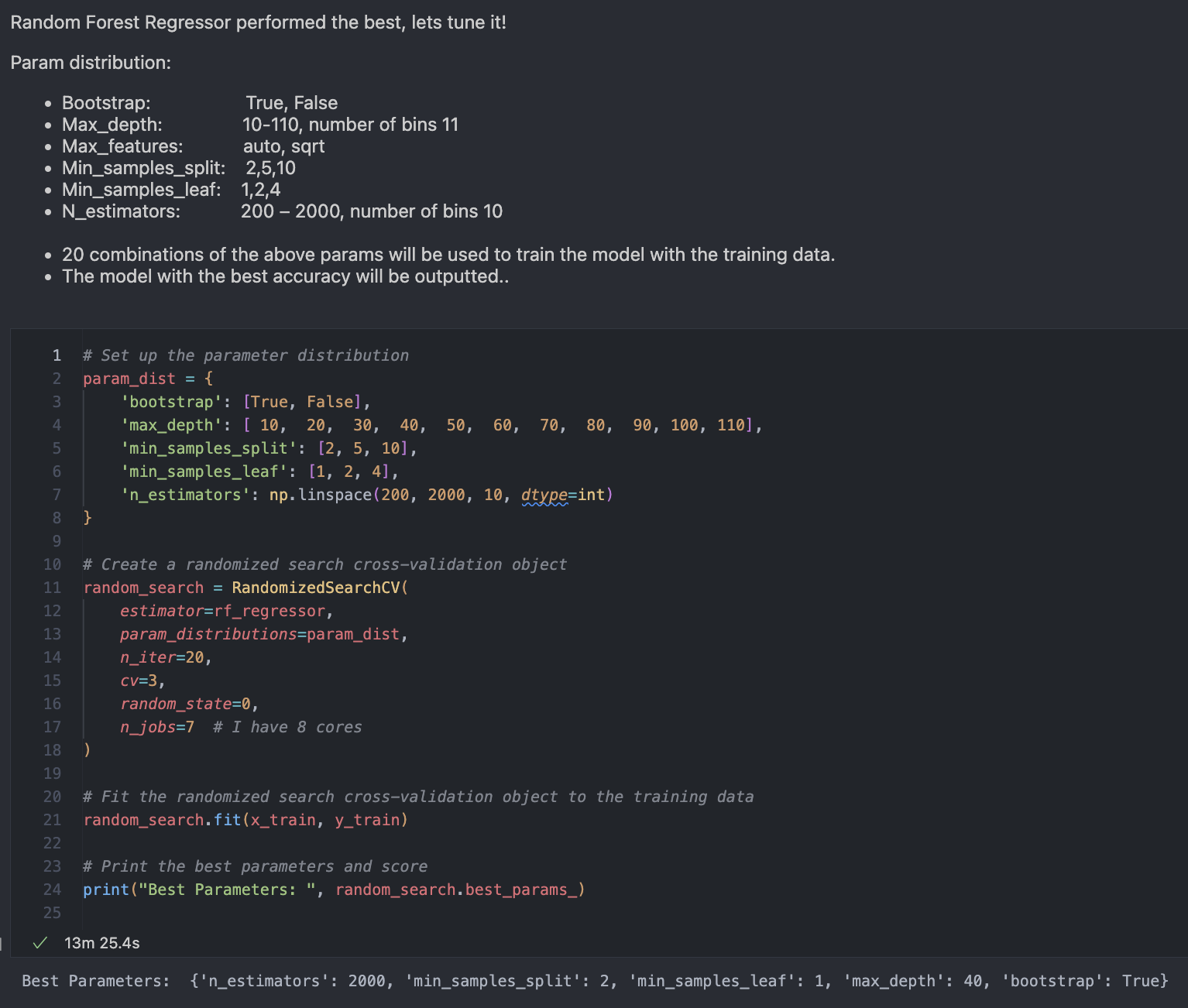
Random Forest Regressor had the best results, but let's see if we can do better.
An iterative randomized search was performed on the RF model. This approach is fast and still ensures that we are sampling the parameter space well by doing 20 different attempts.
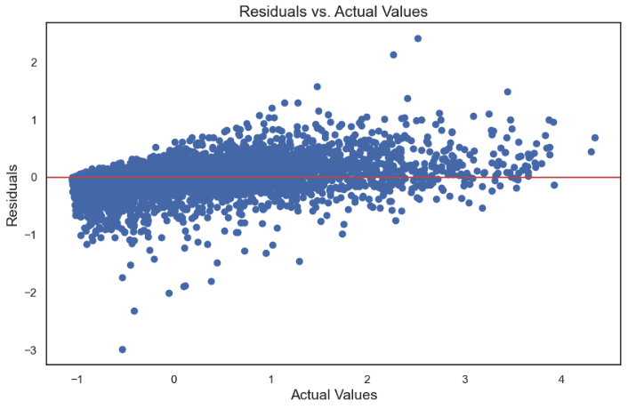
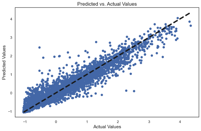
Now with the best model selected, and parameters tuned, we can evaluate the model and see how it performed.

- The residuals are centered around the zero line, which suggests that, on average, the model predictions are fairly accurate.
- The spread of residuals appears to be consistent across the range of actual values, indicating that the variance of the errors is constant (homoscedasticity). This is a good sign, as it means the model is equally reliable across the entire range of data.
- There are no clear patterns or trends in the residuals, which suggests that the model isn’t systematically over- or under-predicting at different values of the actual variable.
- The fact that there are a few residuals that lie quite far from the zero line, especially for higher actual values, indicates the presence of some outliers or extreme values that the model is not predicting well.
- The points seem more dispersed at the higher end of actual values. This suggests that the model may be more accurate for lower values and less accurate for higher values.
- There aren't many points that are extreme outliers, but the spread does increase with the value of the target, which might suggest heteroscedasticity, a condition where the variance of errors differs across the range of the predictor variable.
Overall, both the residual plot and the predicted versus actual values plot, our model seems to generally predict values that are close to the actual values. However, the model’s performance decreases with higher actual values, as indicated by the spread and pattern of residuals, suggesting potential areas for improvement, such as addressing heteroscedasticity or model fit.
Using our random forest regressor we can identify which variables are the most important for making accurate predictions, the mean gini decrease.
Not surprisingly we can see that:
- More rides in higher temperatures
- Less rides in higher humidities
- More rides during rush hour times
Now let's visualize the two most important variables and thier relationship towards the number of riders.
