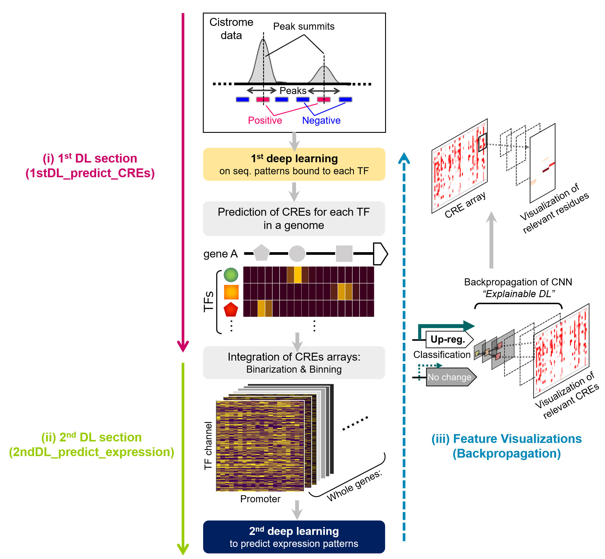
Deep learning on cis-decoding with cistrome datasets

STRUCTURE

(i). Training of TFs recognition patterns from cistrome datasets [on directory “1stDL_predict_CREs”]

(ii). Deep learning for binary classification of expression patterns [on directory “2ndDL_predict_expression”]

(iii). Feature visualization [on directory “Backpropagation”])

(i). Training of TFs recognition patterns from DAP-Seq

Extract fragments including significant peak from DAP-Seq (NOTE: the length should be identical), to convert into simple text files. If you target 31-bp tiles, save as .txt like,
```
 ATGCGTGCGTGCGTGGCTGCAATGTGCAAAT 
 GGGTACTAGCTTGTATATAGCAAATATAGCA 
```

Training/validation by a fully-connected model

 python FC-cistrome-training.py [-p] [-n] [-o] [-e] [-l] 
 
 option:
     "-p", help="File path to positive DNAs" 
     "-n", help="File path to negative DNAs" 
     "-o", help="output prefix" 
     "-e", help="epoch numbers" 
     "-l", help="DNA length"

→ Output “.h5 file” with ROC-AUC data.

Detection of prediction (of each TF biding) in the target promoter sequences in bin sliding-windows.

Target promoter sequences should be in fasta format.

 python MultiSeq_CREs_prediction_walking.py [-f] [-m] [-w] [-b] [-o] 

 option:
     "-f", help="File path to fasta" 
     "-m", help="File path to HDF5 or H5 model" 
     "-w", help="walk bp size" 
     "-b", help="bin bp size" (should be same as the tile set above)
     "-o", help="output file name"

→ Output “wOTU_XXX(out)” with each target info as OTUs.

Conversion to binary CRE arrays in bins

 python BinIntg2BinaryArray.py [-i] [-b] [-t] [-o] 
 
 option:
     "-i", help="File path to input" 
     "-b", help="bin size" 
     "-t", help="confidence threshold (0-1)" 
     "-o", help="output file name"

With 2-bp walking size in the previous step (MultiSeq_CREs_prediction_walking.py), “-b 25” produces an array with 50-bp bins.

If input file is like

 geneA	0.1	0.4	0.9	0.1	0.1	0.0	0.2	1.0	0.9

-b 3 -t 0.8 produces

 geneA	1   0   1

(ii). Deep learning for binary classification of expression patterns

Use “2ndDL_predict_expression” directory.

Move all of the data including transitions of the predicted TF-binding sites for all target promoters, into “raw_data”.
python make_dataset.py (--raw_data_root [directory including data])

→ Output compiled data (train_00/, train_01/…) into /gene_dataset

Make target binary expression pattern” (with the identical OTU names).

target binary expression pattern file (with a specific name) is like (tab-delimited),

 geneA	0 
 geneB	1 
 geneC	0 
 geneD	0 
 geneE	1

Now, the file/code structure is like,

 /root 
 ├ 1dCNN_CisDecoding_training_basic.py 
 ├ data_utils/generator.py 
 ├ make_dataset.py 
 ├ gene_dataset/ 
 │       ├ train_00/ 
 │       │   ├ >XXX.npy 
 │       │   ├ >YYY.npy 
 │       │   ⋮ 
 │       │   └ >ZZZ.npy 
 │       ├ train_01/ 
 │       ├ train_02/ 
 │       ⋮ 
 │       └ train_09/ 
 │     
 ├ binary_expr_pattern file (a specific name) 
 ├ cnn_models/cnn_model_bisic.py

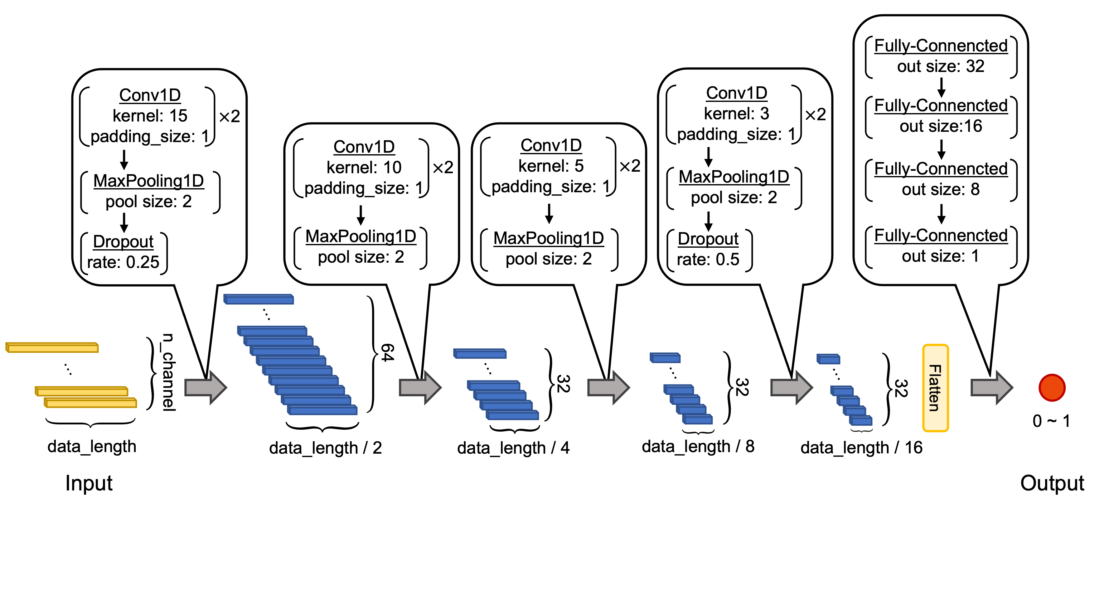
python 1dCNN_CisDecoding_training_basic.py [--n_channel] [--data_length] [--batch_size] [--epochs] [--val_rate] [--shuffle] [--class_weight] [--target_file] [--learning_rate] [--out_file] [--prediction_file]

 option:
     --n_channel', default=50, help='number of channels.' 
     --data_length', default=20, help='length of sequence.' 
     --batch_size', default=156, help='batch size for training.' 
     --epochs', default=10, help='number of epochs for training.' 
     --val_rate', default=0.3, help='rate of validation data.' 
     --shuffle', default=True, help='phenotype data training shuffle' 
     --class_weight', default=5, help='class-weight or positive sample imbalance rate' 
     --target_file', default='BRup.txt', help='phenotype data file' 
     --learning_rate', default=0.0001, help='learning rate' 
     --out_file', default='model.h5', help='output model file name' 
     --prediction_file', default='prediction.txt', help='output prediction confidence file name'

→ Output trained h5 file, list for prediction confidence in validation datasets, ROC-AUC value and curve, and confusion matrix.

(iii) Feature visualization by Guided Backpropagation (other methods are also applicable)

Use “Backpropagation” directory. This step requires “jupyter notebook”, handling “ipynb” format

(iii-1) Feature visualization in the 2nd DL framework: expr pattern -> CREs

GuidedBackProp_CisDecode_batch.ipynb (need “visualizations_forCisDecode.py” and “helper_forCisDecode2.py” in the same directory.) Open jupyter, and run the ipynb file.

NOTE: At the third cell given below, we may have to repeat runs of this cell until the “dense” name is properly changed (expect 4-times)

 partial_model = Model(
     inputs=model.inputs,
     outputs=iutils.keras.graph.pre_softmax_tensors(model.outputs),
     name=model.name,
 )
 partial_model.summary()

Need the trained prediction model “XXX.h5”, and “YYY.npy” for the objective genes, which have been made in the “make_dataset.py” section in the section (ii) above.
The objective gene files (in npy format) need to be located on “select_GBP” directory.

(iii-2). Feature visualization in the 1st DL framework: high confidence CREs -> nucleotide residues

GuidedBackprop_CREs-prediction.ipynb (need “visualizations_forCisDecode.py” and “helper_forCisDecode2” in the same directory.)
Need a prediction model “ZZZ.h5” for each TF channel, which has been made in the section (i), and “fragments list” for the objective tiles, which would be made from a promoter sequence.