Steps to run the code:
- git clone https://github.com/omar-florez/scratch_mlp/
- python scratch_mlp/scratch_mlp.py
A neural network is a clever arrangement of linear and non-linear modules. When we choose and connect them wisely, we have a powerful tool to approximate any mathematical function. For example one that separates classes with a non-linear decision boundary.
A topic that is not always explained in depth, despite of its intuitive and modular nature, is the backpropagation technique responsible for updating trainable parameters. Let’s build a neural network from scratch to see the internal functioning of a neural network using LEGO pieces as a modular analogy, one brick at a time.
Code implementing this can be found in this repository: https://github.com/omar-florez/scratch_mlp
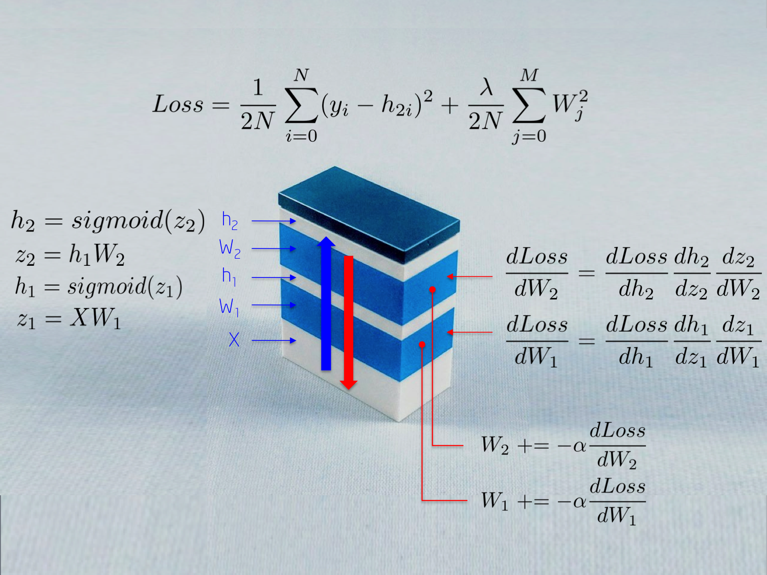
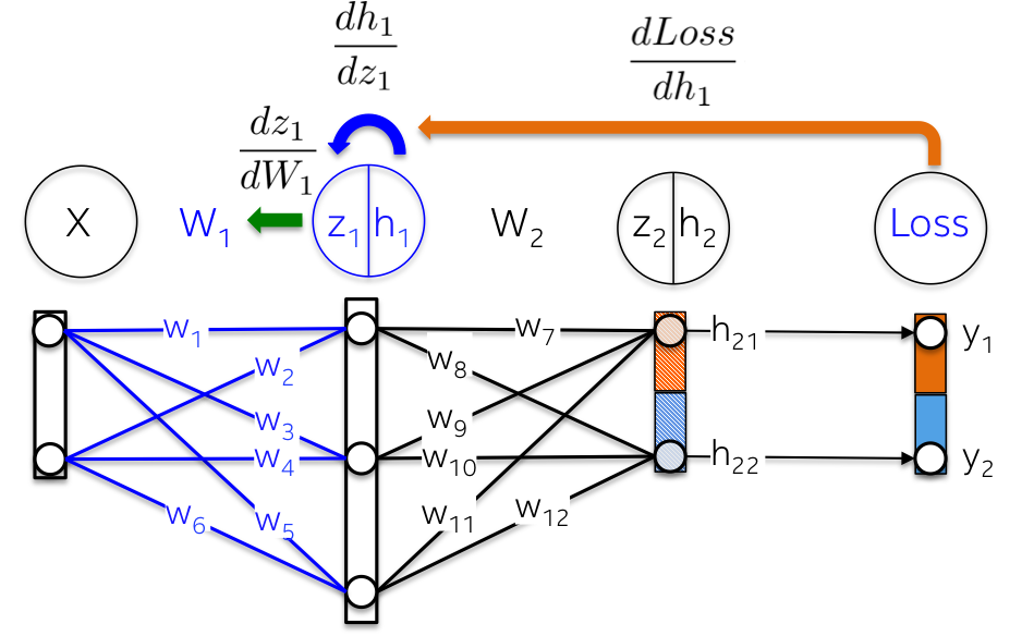
The above figure depicts some of the Math used for training a neural network. We will make sense of this during this article. The reader may find interesting that a neural network is a stack of modules with different purposes:
- Input X feeds a neural network with raw data, which is stored in a matrix in which observations are rows and dimensions are columns
- Weights W1 maps input X to the first hidden layer h1. Weights W1 works then as a linear kernel
- A Sigmoid function prevents numbers in the hidden layer from falling out of range by scaling them to 0-1. The result is an array of neural activations h1 = Sigmoid(WX)
At this point these operations only compute a general linear system, which doesn’t have the capacity to model non-linear interactions. This changes when we stack one more layer, adding depth to this modular structure. The deeper the network, the more subtle non-linear interactions we can learn and more complex problems we can solve, which may explain in part the rise of deep neural models.
If you understand the internal parts of a neural network, you will quickly know what to change first when things don't work and define an strategy to test invariants and expected behaviors that you know are part the algorithm. This will also be helpful when you want to create new capabilities that are not currently implemented in the ML library you are using.
Because debugging machine learning models is a complex task. By experience, mathematical models don't work as expected the first try. They may give you low accuracy for new data, spend long training time or too much memory, return a large number of false negatives or NaN predictions, etc. Let me show some cases when knowing how the algorithm works can become handy:
- If it takes so much time to train, it is maybe a good idea to increase the size of a minibatch to reduce the variance in the observations and thus to help the algorithm to converge
- If you observe NaN predictions, the algorithm may have received large gradients producing memory overflow. Think of this as consecutive matrix multiplications that exploit after many iterations. Decreasing the learning rate will have the effect of scaling down these values. Reducing the number of layers will decrease the number of multiplications. And clipping gradients will control this problem explicitly
Let's open the blackbox. We will build now a neural network from scratch that learns the XOR function. The choice of this non-linear function is by no means random chance. Without backpropagation it would be hard to learn to separate classes with a straight line.
To illustrate this important concept, note below how a straight line cannot separate 0s and 1s, the outputs of the XOR function. Real life problems are also non-linearly separable.
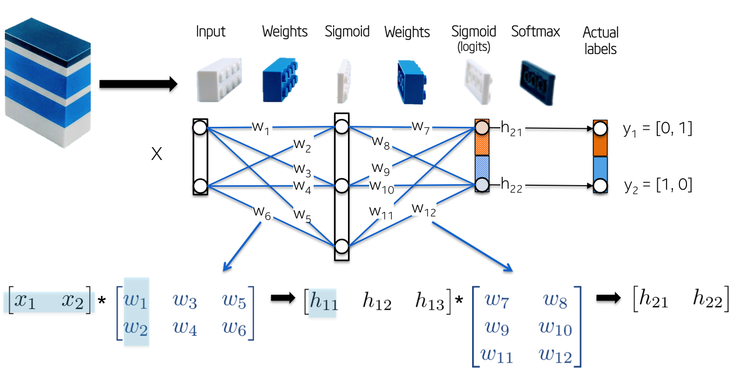
The topology of the network is simple:
- Input X is a two dimensional vector
- Weights W1 is a 2x3 matrix with randomly initialized values
- Hidden layer h1 consists of three neurons. Each neuron receives as input a weighted sum of observations, this is the inner product highlighted in green in the below figure: z1 = [x1, x2][w1, w2]
- Weights W2 is a 3x2 matrix with randomly initialized values and
- Output layer h2 consists of two neurons since the XOR function returns either 0 (y1=[0,1]) or 1 (y2 = [1,0])
More visually:
Let's now train the model. In our simple example the trainable parameters are weights, but be aware that current research is exploring more types of parameters to be optimized. For example shortcuts between layers, regularized distributions, topologies, residual, learning rates, etc.
Backpropagation is a method to update the weights towards the direction (gradient) that minimizes a predefined error metric known as Loss function given a batch of labeled observations. This algorithm has been repeatedly rediscovered and is a special case of a more general technique called automatic differentiation in reverse accumulation mode.
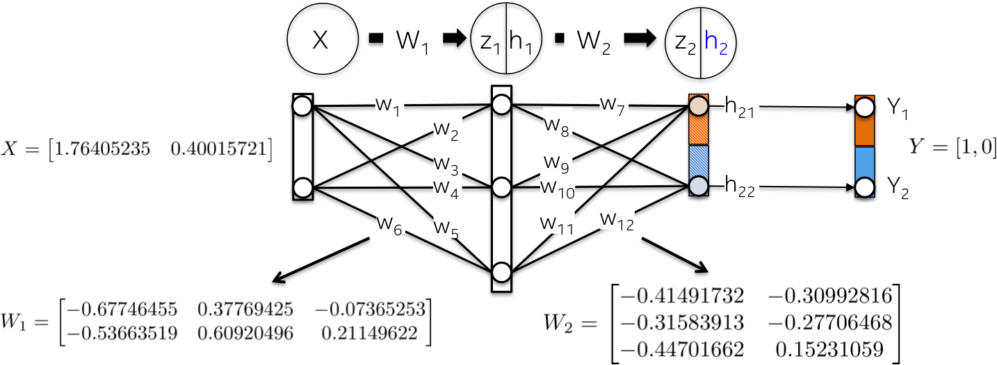
Let's initialize the network weights with random numbers.
This goal of this step is to forward propagate the input X to each layer of the network until computing a vector in the output layer h2.
This is how it happens:
- Linearly map input data X using weights W1 as a kernel:
- Scale this weighted sum z1 with a Sigmoid function to get values of the first hidden layer h1. Note that the original 2D vector is now mapped to a 3D space.
- A similar process takes place for the second layer h2. Let's compute first the weighted sum z2 of the first hidden layer, which is now input data.
- And then compute their Sigmoid activation function. This vector [0.37166596 0.45414264] represents the log probability or predicted vector computed by the network given input X.
Also known as "actual minus predicted", the goal of the loss function is to quantify the distance between the predicted vector h2 and the actual label provided by humans y.
Note that the Loss function contains a regularization component that penalizes large weight values as in a Ridge regression. In other words, large squared weights values will increase the Loss function, an error metric we indeed want to minimize.
The goal of this step is to update the weights of the neural network in a direction that minimizes its Loss function. As we will see, this is a recursive algorithm, which can reuse gradients previously computed and heavily relies on differentiable functions. Since these updates reduce the loss function, a network ‘learns’ to approximate the label of observations with known classes. A property called generalization.
This step goes in backward order than the forward step. It computes first the partial derivative of the loss function with respect to the weights of the output layer (dLoss/dW2) and then the hidden layer (dLoss/dW1). Let's explain in detail each one.
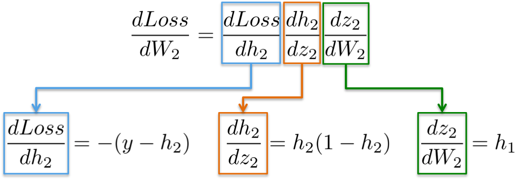
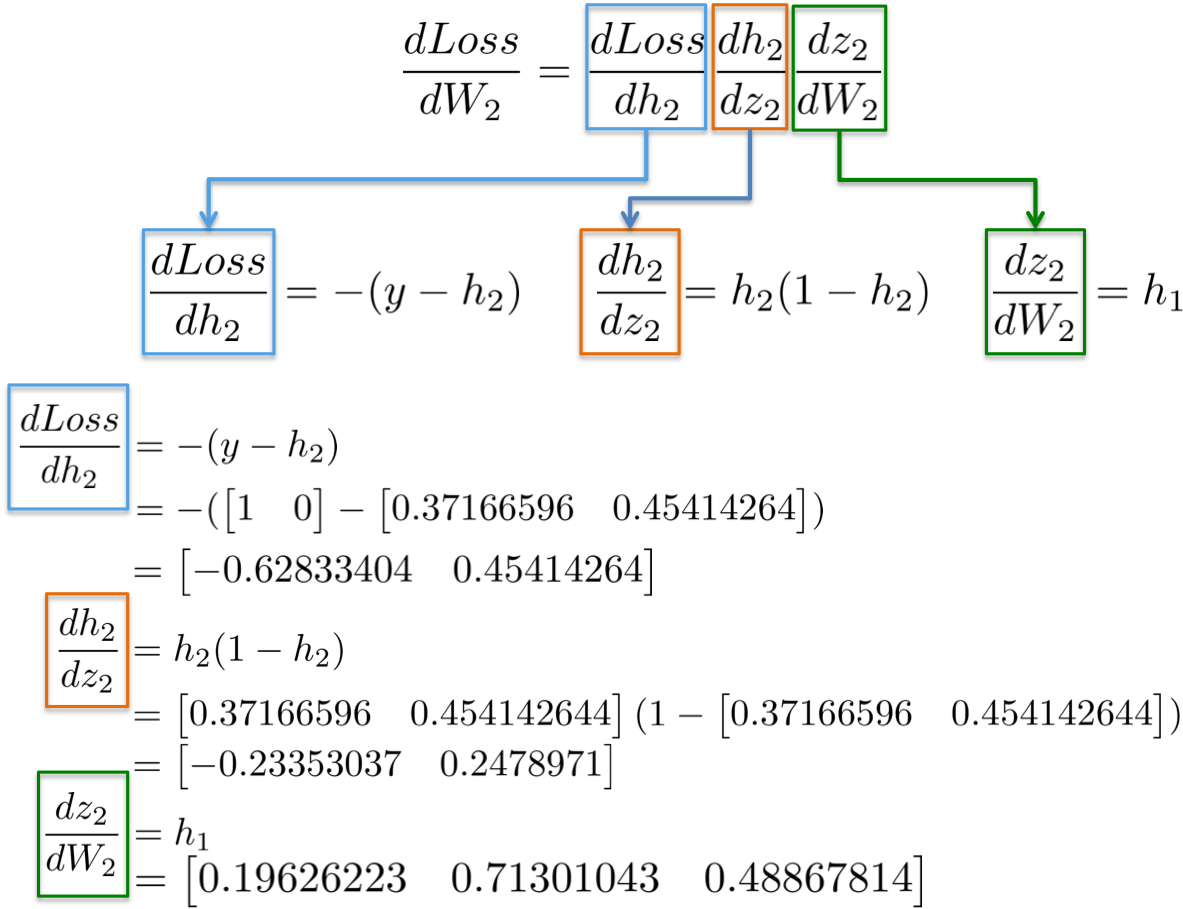
The chain rule says that we can decompose the computation of gradients of a neural network into differentiable pieces:
As a memory helper, these are the function definitions used above and their first derivatives:
| Function | First derivative |
|---|---|
| Loss = (y-h2)^2 | dLoss/dW2 = -(y-h2) |
| h2 = Sigmoid(z2) | dh2/dz2 = h2(1-h2) |
| z2 = h1W2 | dz2/dW2 = h1 |
| z2 = h1W2 | dz2/dh1 = W2 |
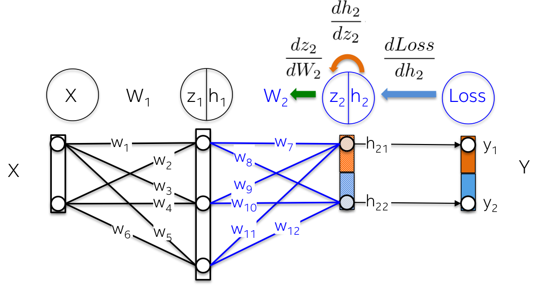
More visually, we aim to update the weights W2 (in blue) in the below figure. In order to that, we need to compute three partial derivatives along the chain.
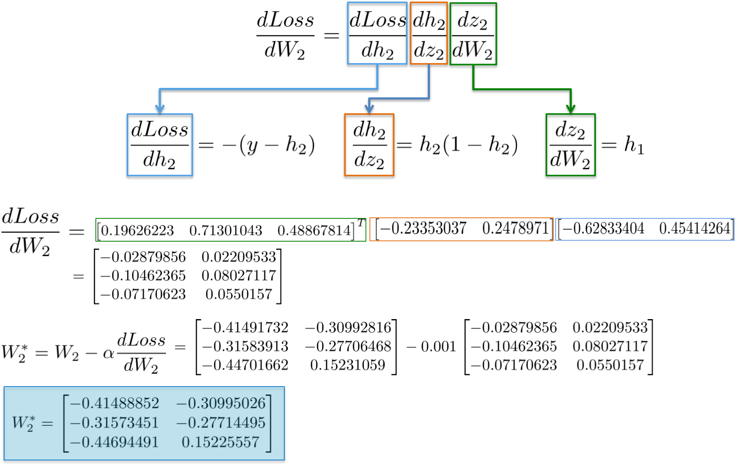
Plugging in values into these partial derivatives allow us to compute gradients with respect to weights W2 as follows.
The result is a 3x2 matrix dLoss/dW2, which will update the original W2 values in a direction that minimizes the Loss function.
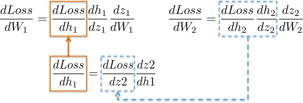
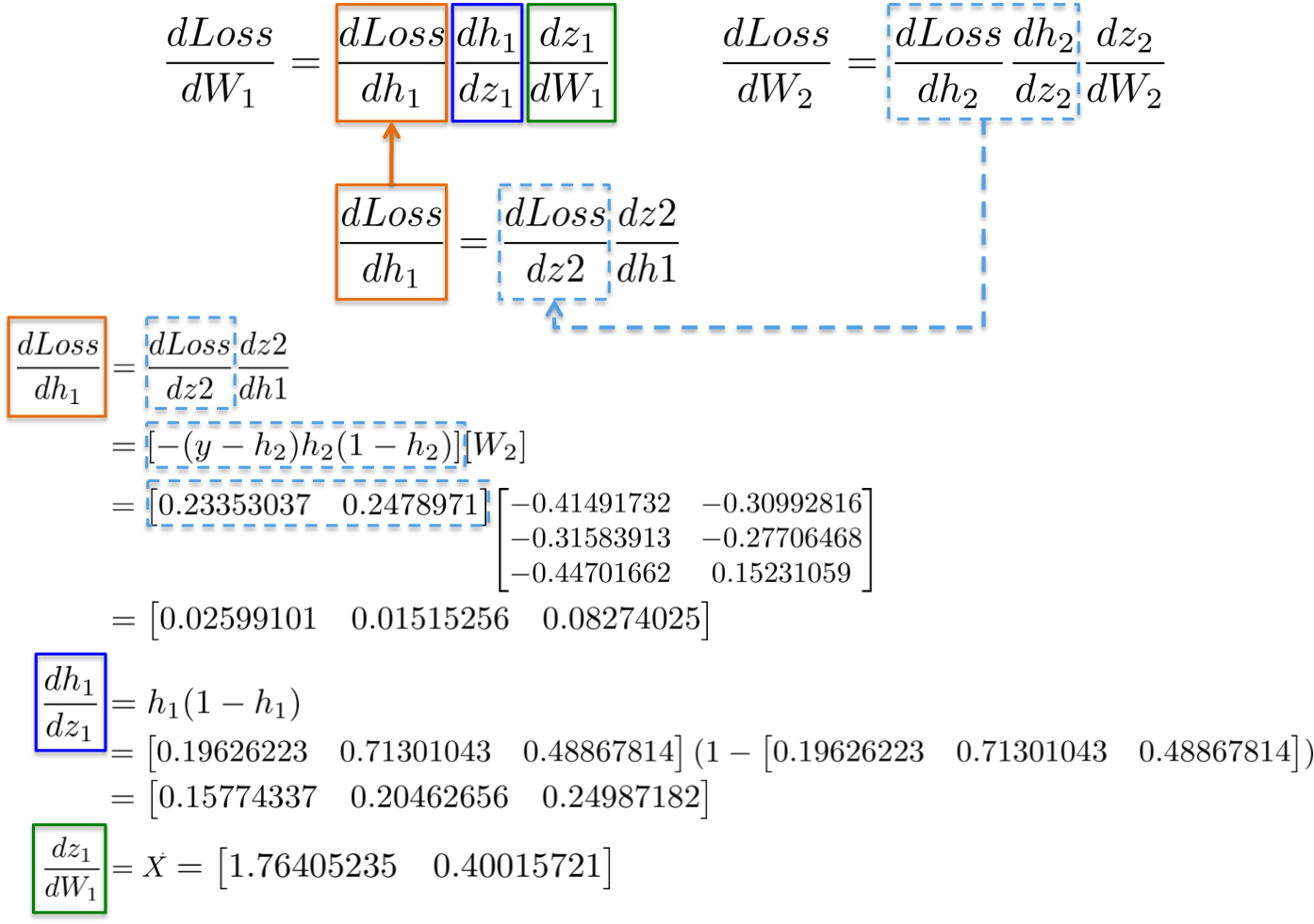
Computing the chain rule for updating the weights of the first hidden layer W1 exhibits the possibility of reusing existing computations.
More visually, the path from the output layer to the weights W1 touches partial derivatives already computed in latter layers.
For example, partial derivatives dLoss/dh2 and dh2/dz2 have been already computed as a dependency for learning weights of the output layer dLoss/dW2 in the previous section.
Placing all derivatives together, we can execute the chain rule again to update the weights of the hidden layer W1:
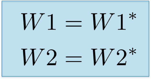
Finally, we assign the new values of the weights and have completed an iteration on the training of network.
Let's translate the above mathematical equations to code only using Numpy as our linear algebra engine. Neural networks are trained in a loop in which each iteration present already calibrated input data to the network. In this small example, let's just consider the entire dataset in each iteration. The computations of Forward step, Loss, and Backwards step lead to good generalization since we update the trainable parameters (matrices w1 and w2 in the code) with their corresponding gradients (matrices dL_dw1 and dL_dw2) in every cycle. Code is stored in this repository: https://github.com/omar-florez/scratch_mlp
See below some neural networks trained to approximate the XOR function over many iterations.
Left plot: Accuracy. Central plot: Learned decision boundary. Right plot: Loss function.
First let's see how a neural network with 3 neurons in the hidden layer has small capacity. This model learns to separate 2 classes with a simple decision boundary that starts being a straight line but then shows a non-linear behavior. The loss function in the right plot nicely gets low as training continues.
Having 50 neurons in the hidden layer notably increases model's power to learn more complex decision boundaries. This could not only produce more accurate results, but also exploiting gradients, a notable problem when training neural networks. This happens when very large gradients multiply weights during backpropagation and thus generate large updated weights. This is reason why the Loss value suddenly increases during the last steps of the training (step > 90). The regularization component of the Loss function computes the squared values of weights that are already very large (sum(W^2)/2N).
This problem can be avoided by reducing the learning rate as you can see below. Or by implementing a policy that reduces the learning rate over time. Or by enforcing a stronger regularization, maybe L1 instead of L2. Exploiding and vanishing gradients are interesting phenomenons and we will devote an entire analysis later.
