This repository accompanies the publication: Verena Praher*, Katharina Prinz*, Arthur Flexer, and Gerhard Widmer, "On the Veracity of Local, Model-agnostic Explanations in Audio Classification: Targeted Investigations with Adversarial Examples". (paper)
(*) equal contribution.
The steps in this README describes how the results can be reproduced in the following steps:
- Setup
- Training the Singing Voice Detector
- Computing Adversaries
- Computing Explanations
- Tables and Visualizations in the Paper
The code was restructured after submission for better readability and we removed some code that was only used for exploration. If you think something is not working as it should be, please let us know :)
The required Python libraries can be found in environment.yml. In addition you need to install audioLIME v0.0.3 by running:
pip install git+https://github.com/CPJKU/audioLIME.git@v0.0.3#egg=audioLIME
Before running the code, please set the variables project_root (results will be stored there) and
dataset_path in svd/path_config.py.
Copy the model model_log_0mean/model.pt into the directory <experiments_path>, such that the
path to the model is <experiments_path>/model_log_0mean/model.pt.
As in the original work of the singing voice detector [1] we use the Jamendo dataset [2] for our experiments. If you want to use this data as well, you can download the data here by choosing the dataset called Jamendo-VAD.
Extracting the archive should give you three folders audio (containing the audio),
filelist (containing the train/validation/test splits) and
labels (containing the annotations for every song). These folders should be moved into dataset/jamendo,
in which already a folder models (containing a pretrained model) should be located.
This work is based on the Singing Voice Detector proposed by Schlüter and Lehner [1]. Our code is therefore strongly based on this repository.
For training a singing voice detector, you can call e.g.,
python -m svd.train dataset/jamendo/models/new/model.pt --dataset-path=dataset/jamendo/audio --validate --save-errors
Here you first need a path to where you want to store the new model at, and a valid
path pointing to the data. The remaining arguments used above indicate that we compute
the validation error during training, and that errors for different epochs are stored.
For more information and the remaining available arguments, see svd/train.py.
Hyperparameters for training can be configured e.g., by modifying svd/default.vars.
To compute predictions for validation (and test) data, run
python -m svd.predict dataset/jamendo/models/model_log_0mean/model.pt dataset/jamendo/models/model_log_0mean/pred.npz --dataset-path=dataset/jamendo/audio --vars=dataset/jamendo/models/model_log_0mean/model.vars
Here the first path should point to the file where the model weights have been stored
at. Make sure you also use the same configurations as during training, e.g.,
by passing an appropriate vars file .
Furthermore, an .npz file to store the predictions in is required. Also adapt the path
pointing to the data if necessary. For more information about all remaining arguments,
see svd/predict.py.
To evaluate previously obtained predictions, you can call e.g.,
python -m svd.eval dataset/jamendo/models/model_log_0mean/pred.npz --dataset-path=dataset/jamendo/audio --auroc
This call requires the path to the file where the predictions were stored previously,
and again the path pointing to the data. --auroc computes the area under the receiver operating characteristic
in addition to other metrics. For more information on the remaining arguments, see svd/eval.py.
The final classification error of the singing voice detector (in percent) on the Jamendo test data, given as the mean ± standard deviation over 5 different runs, is 11.54 ± 0.96. Furthermore, recall and specificity over 5 runs are 89.61 ± 1.71 and 87.46 ± 1.00 respectively.
To compute adversaries on the raw waveform, you can call e.g.,
python -m svd.adversaries.raw_attack dataset/jamendo/models/model_log_0mean/model.pt --adv-dir=dataset/jamendo/adversaries --dataset-path=dataset/jamendo/audio --vars=dataset/jamendo/models/model_log_0mean/model.vars --test --threshold=0.51
The most important parameter is the first one, where the path to the model under attack should be stated. The second required parameter is the path to where the adversarial examples should be stored. Finally, please also set the path to where the data is located, and define the model parameters accordingly (e.g., here we linked the file containing variables we used during training).
The remaining two arguments
in this example are --test, which indicates that we compute adversaries for test-data
instead of validation data, and --threshold, which is an optimised threshold for classifying
singing voice with the pre-trained model we provide.
For more details and a complete set of parameters, please refer to svd/adversaries/raw_attack.py.
Note that per default, the attack parameters defined in adv_default.vars are used -
feel free to change them!
To compute adversaries on the spectrogram instead, change the above command as follows:
python -m svd.adversaries.spec_attack dataset/jamendo/models/model_log_0mean/model.pt --adv-dir=dataset/jamendo/adversaries --dataset-path=dataset/jamendo/audio --vars=dataset/jamendo/models/model_log_0mean/model.vars --test --threshold=0.51
Once more, the attack parameters are defined in adv_default.vars, and all arguments
to run the attack are as for the attack on raw audio (see svd/adversaries/raw_attack.py).
Note, that the success rate of the adversarial attacks is relatively low when looking at the number of excerpts we successfully flipped. We assume that this is due to the fact that we decided to store entire adversarial songs instead of adversarial excerpts; that way, we make adversarial changes at a file-level, but have our adversarial targets at an excerpt-level. In other words, a single change to the file can influence multiple overlapping excerpts at the same time.
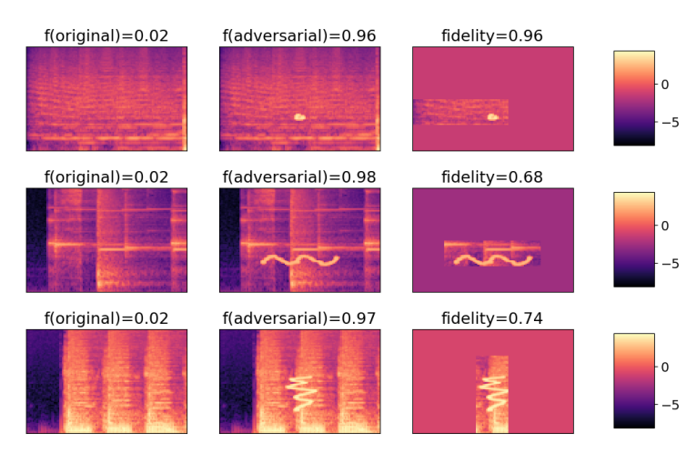
We stored a set of spectrograms, for which we modified the prediction from "no sing"
to "sing" by drawing on them, in horses/horses1.pt, horses/horses2.pt, and horses/horses3.pt.
To compute explanations, call:
python -m svd.explanations.compute_and_store_horse_explanations --which_horses horses1 --baseline mean
python -m svd.explanations.compute_and_store_horse_explanations --which_horses horses2 --baseline mean
python -m svd.explanations.compute_and_store_horse_explanations --which_horses horses3 --baseline mean
First pick 10 adversaries per attack type (spec/wave) and adversarial direction (sing → no sing; no sing → sing).
python -m svd.explanations.pick_and_store_adversaries --attack_type wave --subset test --target 1
python -m svd.explanations.pick_and_store_adversaries --attack_type spec --subset test --target 1
python -m svd.explanations.pick_and_store_adversaries --attack_type wave --subset test --target 0
python -m svd.explanations.pick_and_store_adversaries --attack_type spec --subset test --target 0
To compute explanations for the selected adversarial examples, run the following:
python -m svd.explanations.compute_and_store_explanations --attack_type spec --subset test --baseline mean --target 1
python -m svd.explanations.compute_and_store_explanations --attack_type wave --subset test --baseline mean --target 1
python -m svd.explanations.compute_and_store_explanations --attack_type wave --subset test --baseline mean --target 0
python -m svd.explanations.compute_and_store_explanations --attack_type spec --subset test --baseline mean --target 0
Here we summarize how to reproduce the figures and tables in our paper and the main conclusions:
- Figure 1: "Obvious" causes for predictions can be detected with high fidelity.
To reproduce the figure, run:
python -m svd.visualizations.create_horse_figure --which_horses horses1 --horse_index 1
python -m svd.visualizations.create_horse_figure --which_horses horses2 --horse_index 6
python -m svd.visualizations.create_horse_figure --which_horses horses3 --horse_index 4
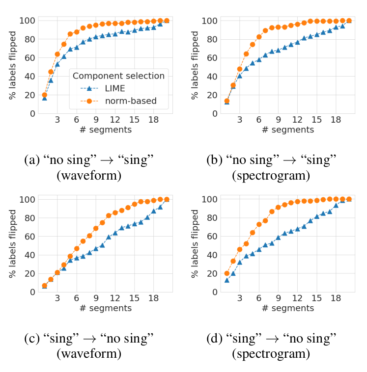
- Figure 2: When using a varying number of interpretable features, we detect fewer "correct" segments than when simply taking the same number of segments with the highest magnitude.
To reproduce the figure, run:
python -m svd.visualizations.create_flip_count_figure --attack_type spec --subset test --baseline mean --target 0
python -m svd.visualizations.create_flip_count_figure --attack_type spec --subset test --baseline mean --target 1
python -m svd.visualizations.create_flip_count_figure --attack_type wave --subset test --baseline mean --target 0
python -m svd.visualizations.create_flip_count_figure --attack_type wave --subset test --baseline mean --target 1 --plot_legend
The above calls will also output the numbers reported in Table 1:
- Table 1: When computing the 3 most relevant interpretable features with LIME, we detect segments that are able to flip the label for only 21-53% of the excerpts.
- Table 2: When using all interpretable features that received a positive weight, we detect fewer "correct" segments than when taking the same number of segments with the highest magnitude.
The values are computed by the following script:
python -m svd.explanations.compute_results_table_2 --attack_type spec --baseline mean --target 0
python -m svd.explanations.compute_results_table_2 --attack_type spec --baseline mean --target 1
python -m svd.explanations.compute_results_table_2 --attack_type wave --baseline mean --target 0
python -m svd.explanations.compute_results_table_2 --attack_type wave --baseline mean --target 1
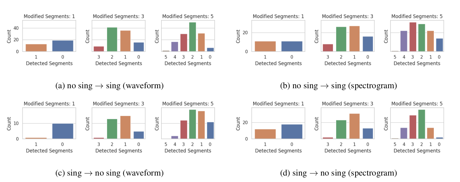
- Figure 3: In a setting where we only add partial perturbations, only few segments are correctly detected.
To reproduce this figure first run:
python -m svd.explanations.explain_subset_perturbations --attack_type wave --subset test --baseline mean --target 1
python -m svd.explanations.explain_subset_perturbations --attack_type spec --subset test --baseline mean --target 1

python -m svd.explanations.explain_subset_perturbations --attack_type wave --subset test --baseline mean --target 0
python -m svd.explanations.explain_subset_perturbations --attack_type spec --subset test --baseline mean --target 0
And then run:
python -m svd.visualizations.create_subset_perturbation_figure --attack_type spec --subset test --baseline mean --target 0
python -m svd.visualizations.create_subset_perturbation_figure --attack_type spec --subset test --baseline mean --target 1
python -m svd.visualizations.create_subset_perturbation_figure --attack_type wave --subset test --baseline mean --target 0
python -m svd.visualizations.create_subset_perturbation_figure --attack_type wave --subset test --baseline mean --target 1
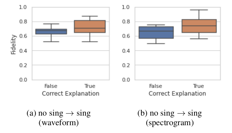
- Figure 4: Based on the fidelity score it is impossible to judge the quality of an explanation.
python -m svd.visualizations.create_fidelity_figure --attack_type wave --target 1
python -m svd.visualizations.create_fidelity_figure --attack_type spec --target 1
[1] J. Schlüter and B. Lehner, “Zero-Mean Convolutions for Level-Invariant Singing Voice Detection,” in Proceedings of the 19th International Society for Music Information Retrieval Conference, ISMIR 2018, Paris, France, September 23-27, 2018, pp. 321–326.
[2] M. Ramona, G. Richard, and B. David, “Vocal Detection in Music with Support
Vector Machines,” in Proceedings of the IEEE International Conference on Acoustics,
Speech, and Signal Processing, ICASSP 2008, Las Vegas, Nevada, USA.
IEEE, 2008, pp.1885–1888.


