Download link for trained model weights : https://drive.google.com/file/d/1hE9It0ZOOeIuSFvt6GdiR_0cq9inWdTy/view?usp=sharing
With the huge success of deep learning in the field of computer vision, there is rising awareness of its application in medical image. Detection of brain tumor using a segmentation approach is critical in cases, where survival of a subject depends on an accurate and timely clinical diagnosis. Gliomas are the most commonly found tumors having irregular shape and ambiguous boundaries, making them one of the hardest tumors to detect. We present a fully automatic deep learning approach for brain tumor segmentation in multi-contrast magnetic resonance image. The proposed approach is based on fully convolutional network (FCN) and using U-net as the model. Using the dataset provided for the Brain Tumor Segmentation (BraTS) Challenge by the Medical Image Computing and Computer Assisted Intervention (MICCAI) society. Our proposal was validated in the BraTS2018 leaderboard dataset and achieve mean Dice Similarity Coefficient metric of 0.87 in the full tumor region, 0.76 in the tumor core region and 0.71 in the enhancing tumor region, also median Dice Similarity Coefficient metric of 0.90, 0.84, 0.80 for the full tumor, tumor core, and enhancing tumor, respectively.
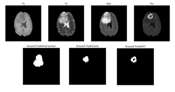
Magnetic resonance imaging (MRI) is commonly used in medical image for analysis of brain tumors. MRI is a non-invasive system, which can be utilized alongside with other imaging modalities, such as computed tomography (CT), positron emission tomography (PET) to give accurate data for brain tumor structure. However, using these systems alongside MRI is expensive and, in some of the case, can be invasive (e.g. PET). Therefore, different MR that are non-invasive and image both structure and functions are mostly used for brain imaging. MRI machines themselves come with different configurations and produce images with varying intensities. This makes tumor detection a difficult task when different MRI configurations (such as magnetic field strength 1.5, 3 or 7 Tesla) and the acquisition protocol (field of view value, voxel resolution, gradient strength, b0 value, etc.) are used. These configurations have different intensity values across voxels, which result in the same tumorous cells may have different grayscale values when pictured in different hospitals. MRI can show different tissue contrasts through different pulse sequences, making it an adaptable and widely used imaging technique for visualizing regions of interest in the human brain. MRI modalities are combined to produce multi-modal images giving more information about irregular shaped tumors, which are difficult to localize with a single modality. These modalities include T1-weighted MRI (T1), T1-weighted MRI with contrast enhancement (T1c), T2-weighted MRI (T2) and T2-weighted MRI with fluid attenuated inversion recovery (T2-Flair). This multi-modal data contains information that can be used for tumor segmentation with significant improvement in performance. Figure 1 shows an axial slice of the four standard sequences for a glioma patient including manually drawn tumor regions. T1-weighting is the most commonly used sequence for the structural analysis; it also allows for an easy annotation of the healthy tissues. In T1-weighted contrast-enhanced images (gadolinium-DTPA), the tumor borders appear brighter because the contrast agent accumulates there due to the disruption of the blood–brain barrier in the proliferative tumor region. In this sequence, the necrotic and the active tumor region can be distinguished easily. In T2-weighted MRI, the edema region, which surrounds the tumor, appears bright. T2FLAIR (FLAIR) is a special sequence, which helps in separating the edema region from the cerebrospinal fluid (CSF) because the free water signal is suppressed. The radiological definition of the tumor margins in the clinical context are often manually determined by the radiologist on the T2 and post-gadolinium T1 images by thresholding boundaries between T2 hyperintense/T1 contrast-enhanced lesions and the surrounding healthy tissue to define the outer margins of a tumor.
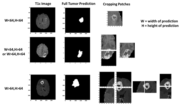
Figure 1: One axial slice of an MR image of a high-grade glioma patient. From left to right in row 1: T1-weighted image, T2-weighted image, T2-FLAIR-weighted image T1-weighted image with contrast enhancement. In row 2, showing the three sub-region ground truth labeled by exports. Figure 2: The overview of the proposed approach for brain tumor segmentation.At first, we use only one U-net model to do three different segmentation tasks (Full Tumor, Tumor Core, Enhancing Tumor), the result of full tumor is promising but the rest of two is not good. We find out that the problem is because the tumor core and enhancing tumor are too small compare to the whole brain, which means the pixel number of these two labels are too little (average 0.75% for tumor core and 0.45% for enhancing tumor per slice). Therefore, the data imbalanced problem cause that model tend to predict “no tumor” but still can get good result. According to Figure 1, we knew that tumor core must be inside of edema, and enhancing tumor is part of tumor core. To solve the problem, we use the advantage of full tumor prediction and calculating the center point of full tumor, then use the center point to crop out the training data for tumor core and enhancing tumor (shown in Figure 3). The number of cropping depend on the size of full tumor and we even crop the overlap part to do data-augmentation, cropping size is 64x64 fixed. After cropping, the ratio of tumor core and enhancing tumor have achieved average 12.7% and 7.6% per training patch.
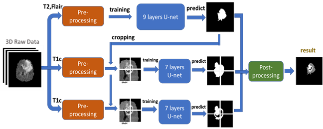
Figure 3: The cropping method we proposed for improving the performance of tumor core and enhancing tumor segmentation. Cropping the T1c image according to center point of full tumor prediction. The patch size is 64x64 and if the tumor size is bigger than 64x64, we crop more than 1 patch.Then we put the 64x64 training data into another U-net model to train and predict. The result of tumor core prediction and enhancing tumor prediction will be paste back to original full tumor prediction according the center point we got. Fig. 4 present the flowchart of the proposed approach. Instead of using all MRI modalities as, we only use T2 and Flair data for full tumor segmentation and only T1ce for tumor core/enhancing tumor segmentation to accelerate training. According to, to those radiologists, the edema was segmented primarily from T2 images and FLAIR was used to cross-check the extension of the edema and discriminate it against ventricles and other fluid-filled structures. Tumor core and enhancing tumor was both segmented by evaluating hyper-intensities in T1ce images.
Figure 4: we use T2 and Flair image (after pre-processing) as input to a 9 layers U-net for full tumor segmentation. Then using the full tumor prediction to crop out the training patches from T1c image (after pre-processing). These training patches are put in to two 7 layers U-net for tumor core segmentation and enhancing tumor segmentation. Then we combine all three predictions by post-processing and getting final results.The MRI images was already skull stripped and resampled to 1mm3 resolution as we got the dataset. No non-uniform intensity normalization algorithm or non-parametric algorithm has been used to correct for intensity non-uniformities caused by the inhomogeneity of scanner’s magnetic field, because it will be obliterated the T2-Flair signal. We use SimpleITK. to read the NIFTI format data. and covert to numpy array format. The data size of each subject is 240x240x155, we only pick the 60-120th axial slices as training data due to the rest part of brain is very unlikely to have any tumor. The slices are then zero-mean normalized using the mean and standard deviation.
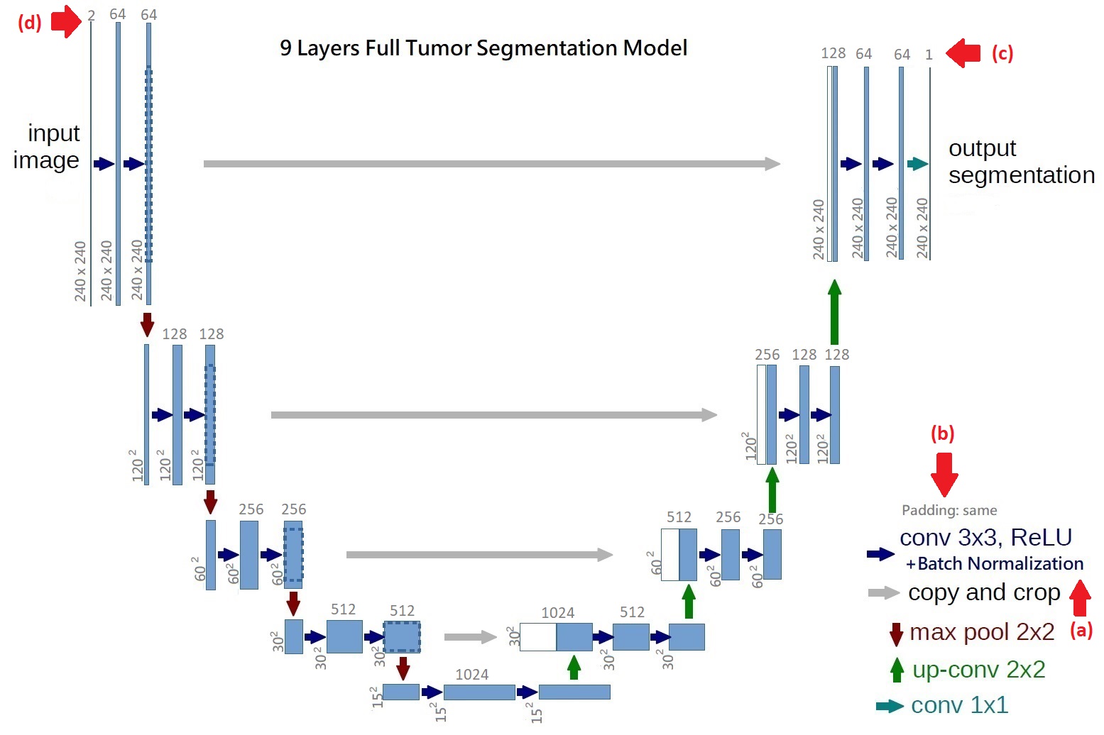
Our brain tumor segmentation model consists two stages. Firstly, we use a 9 layers U-net like architecture to segment full tumor. Secondly, using segmentation result as input for two 7 layers U-net like architectures to segment tumor core and enhancing tumor. The architecture of the proposed network is shown in Figure 3-4 and Figure 3-5. The proposed architecture can be considered as an auto-encoder, where a contraction network tries to learn the image features, and an expanding network tries to use these features to reconstruct a low dimensional data representation of image, such as the ground truth of data. The contracting layer consists of stacked convolution/pooling layers, while the expanding network is made up of up-sampling/transposed convolution layers. In order to localize, high resolution features from the contracting path are concatenated with the up-sampled output of different stages. These are called “skip connections”. The advantages of using skip connections are shown in detail by Drozdzal et al. in. They make a distinction between using long skip and short skip, spanning over a single residual block. The difference between original U-net and our U-net is that we connect a batch normalization after each convolution layer to keep the gradient levels controlled, speed up convergence and reduce the effect of internal covariate shift, so that the parameters of the network do not change rapidly during backpropagation. The filter size of convolution layers is 3 x 3 and we use the same padding to keep the output size of convolution layers unchanged, which is also different from original U-net. To increase the receptive filed at the lowest resolution, two layers of convolution/batch normalization are stacked, which is the idea from VGG16. After two convolution layers and batch normalization, a 2 x 2 max-pooling with stride 2 down-sample image size to 1/2. At each down-sampling step they double the number of feature channels. Every step in the expansive path consists of an up-sampling of the feature map followed by a 2x2 transposed convolution (“up-convolution”) that halves the number of feature channels, a concatenation with the correspondingly cropped feature map from the contracting path, and two 3x3 convolutions. Since it is binary segmentation for each model, the final operation is a 1 x 1 convolution with 1 filter, producing binary prediction that 1 is target and 0 is null.
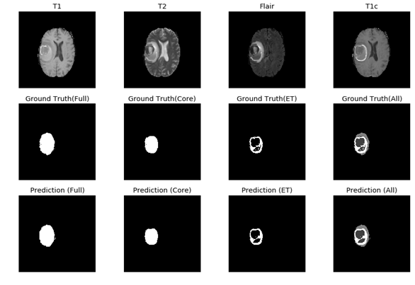
Figure 5: The 9 layers U-net Structure we proposed for full tumor segmentation. There are four differences between our U-net and original U-net (shows by red arrows) [16]. (a) We add batch-normalization layer after each convolution layer. (b) We use same padding in convolution layers to keep the feature map size unchanged. (c) The final convolution filter number is one for binary segmentation. (d) Input channels are two because we use T2 and Flair image for full tumor segmentation. Figure 6: In the first row, we have 4 MRI modalities of a HGG subject from BraTS2015 dataset. Second row shows the ground truth of three different tasks and combination of all three tasks. Third row was the prediction from our method. Figure 7: Result of all three tasks (Green=edema, yellow=enhancing tumor, blue=necrosis and non-enhancing). These are all the 100th slice from different HGG subjects, which are most likely to be center part of brain tumor. The result shows that our method performed well when it comes to core of brain tumor.