WeightWatcher (WW) is an open-source, diagnostic tool for analyzing Deep Neural Networks (DNN), without needing access to training or even test data. It is based on theoretical research into Why Deep Learning Works, based on our Theory of Heavy-Tailed Self-Regularization (HT-SR). It uses ideas from Random Matrix Theory (RMT), Statistical Mechanics, and Strongly Correlated Systems.
It can be used to:
- analyze pre/trained pyTorch, Keras, DNN models (Conv2D and Dense layers)
- monitor models, and the model layers, to see if they are over-trained or over-parameterized
- predict test accuracies across different models, with or without training data
- detect potential problems when compressing or fine-tuning pretrained models
- layer warning labels: over-trained; under-trained
-
Please see our latest talk from the Sillicon Valley ACM meetup
-
Join the Discord Server
-
For a deeper dive into the theory, see our latest talk at ENS
-
and some of the most recent Podcasts:
-
More details and demos can be found on the Calculated Content Blog
And in the notebooks provided in the examples directory
pip install weightwatcherif this fails try
python3 -m pip install --index-url https://test.pypi.org/simple/ --extra-index-url https://pypi.org/simple weightwatcherimport weightwatcher as ww
import torchvision.models as models
model = models.vgg19_bn(pretrained=True)
watcher = ww.WeightWatcher(model=model)
details = watcher.analyze()
summary = watcher.get_summary(details)It is as easy to run and generates a pandas dataframe with details (and plots) for each layer
and summary dictionary of generalization metrics
    {'log_norm': 2.11,      'alpha': 3.06,
      'alpha_weighted': 2.78,
      'log_alpha_norm': 3.21,
      'log_spectral_norm': 0.89,
      'stable_rank': 20.90,
'mp_softrank': 0.52}The watcher object has several functions and analysis features described below
Notice the min_evals setting: the power law fits need at least 50 eigenvalues to make sense but the describe and other methods do not
watcher.analyze(model=None, layers=[], min_evals=50, max_evals=None,
	 plot=True, randomize=True, mp_fit=True, pool=True, savefig=True):
...
watcher.describe(self, model=None, layers=[], min_evals=0, max_evals=None,
         plot=True, randomize=True, mp_fit=True, pool=True):
...
watcher.get_details()
watcher.get_summary(details) or get_summary()
watcher.get_ESD()
...
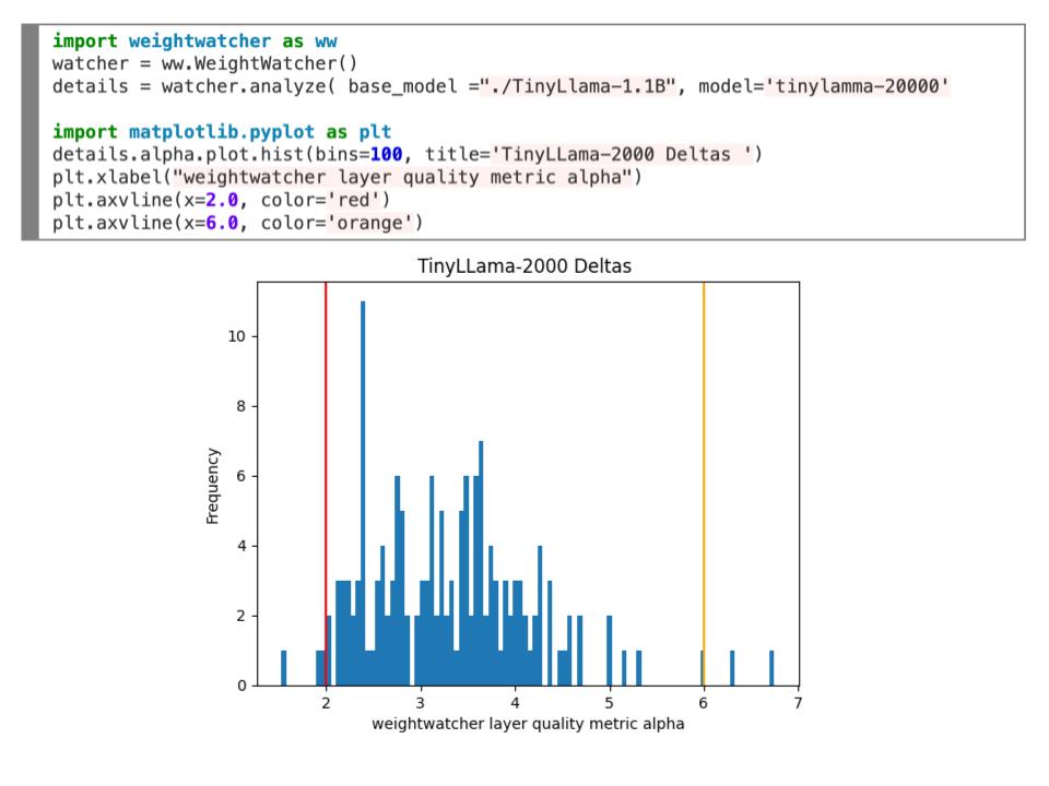
watcher.distances(model_1, model_2)To analyze an PEFT / LORA fine-tuned model, specify the peft option.
-
peft = True: Forms the BA low rank matric and analyzes the delta layers, with 'lora_BA" tag in name
details = watcher.analyze(peft='peft_only') -
peft = 'with_base': Analyes the base_model, the delta, and the combined layer weight matrices.
details = watcher.analyze(peft=True)
The base_model and fine-tuned model must have the same layer names. And weightwatcher will ignore layers that do not share the same name. Also,at this point, biases are not considered. Finally, both models should be stored in the same format (i.e safetensors)
Note: If you want to select by layer_ids, you must first run describe(peft=False), and then select both the lora_A and lora_B layers
WW creates plots for each layer weight matrix to observe how well the power law fits work
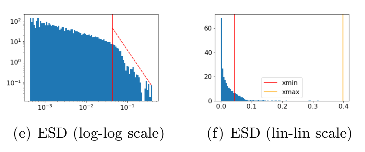
details = watcher.analyze(plot=True)For each layer, WeightWatcher plots the ESD--a histogram of the eigenvalues of the layer correlation matrix X=WTW. It then fits the tail of ESD to a (Truncated) Power Law, and plots these fits on different axes. The summary metrics (above) characterize the Shape and Scale of each ESD. Here's an example:
Generally speaking, the ESDs in the best layers, in the best DNNs can be fit to a Power Law (PL), with PL exponents alpha closer to 2.0.
Visually, the ESD looks like a straight line on a log-log plot (above left).
The goal of the WeightWatcher project is find generalization metrics that most accurately reflect observed test accuracies, across many different models and architectures, for pre-trained models and models undergoing training.
Our HTSR theory says that well trained, well correlated layers should be signficantly different from the MP (Marchenko-Pastur) random bulk, and specifically to be heavy tailed. There are different layer metrics in WeightWatcher for this, including:
rand_distance: the distance in distribution from the randomized layeralpha: the slope of the tail of the ESD, on a log-log scalealpha-hatoralpha_weighted: a scale-adjusted form ofalpha(similar to the alpha-shatten-Norm)stable_rank: a norm-adjusted measure of the scale of the ESDnum_spikes: the number of spikes outside the MP bulk regionmax_rand_eval: scale of the random noise etc
All of these attempt to measure how on-random and/or non-heavy-tailed the layer ESDs are.
alpha:Power Law (PL) exponent
- (Truncated) PL quality of fit
D:(the Kolmogorov Smirnov Distance metric)
(advanced usage)
- TPL : (alpha and Lambda) Truncated Power Law Fit
- E_TPL : (alpha and Lambda) Extended Truncated Power Law Fit
The random distance metric is a new, non-parameteric approach that appears to work well in early testing. See this recent blog post
There re also related metrics, including the new
- 'ww_maxdist'
- 'ww_softrank'
N, M: Matrix or Tensor Slice Dimensionsnum_spikes: number of spikes outside the bulk region of the ESD, when fit to an MP distributionnum_rand_spikes: number of Correlation Trapsmax_rand_eval: scale of the random noise in the layer
The layer metrics are averaged in the summary statistics:
Get the average metrics, as a summary (dict), from the given (or current) details dataframe
details = watcher.analyze(model=model)
summary = watcher.get_summary(model)
or just
summary = watcher.get_summary()The summary statistics can be used to gauge the test error of a series of pre/trained models, without needing access to training or test data.
- average
alphacan be used to compare one or more DNN models with different hyperparemeter settings θ, when depth is not a driving factor (i.e transformer models) - average
log_spectral_normis useful to compare models of different depths L at a coarse grain level - average
alpha_weightedandlog_alpha_normare suitable for DNNs of differing hyperparemeters θ and depths L simultaneously. (i.e CV models like VGG and ResNet)
WeightWatcher (WW) can be used to compare the test error for a series of models, trained on the similar dataset, but with different hyperparameters θ, or even different but related architectures.
Our Theory of HT-SR predicts that models with smaller PL exponents alpha, on average, correspond to models that generalize better.
Here is an example of the alpha_weighted capacity metric for all the current pretrained VGG models.

Notice: we did not peek at the ImageNet test data to build this plot.
This can be reproduced with the Examples Notebooks for VGG and also for ResNet
WeightWatcher can help you detect the signatures of over-fitting and under-fitting in specific layers of a pre/trained Deep Neural Networks.
WeightWatcher will analyze your model, layer-by-layer, and show you where these kind of problems may be lurking.
The randomize option lets you compare the ESD of the layer weight matrix (W) to the ESD of its randomized form.
This is good way to visualize the correlations in the true ESD, and detect signatures of over- and under-fitting
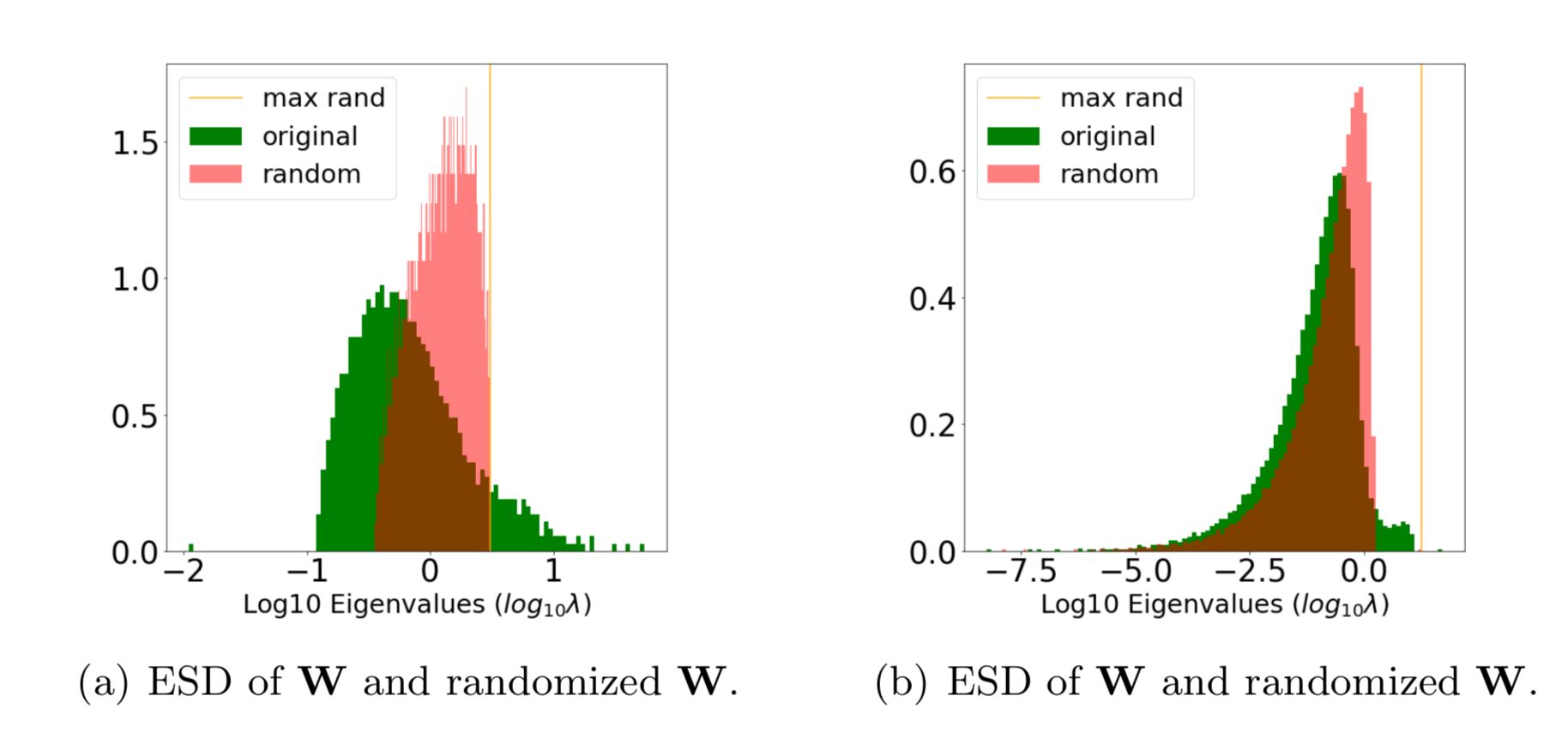
details = watcher.analyze(randomize=True, plot=True)Fig (a) is well trained; Fig (b) may be over-fit.
That orange spike on the far right is the tell-tale clue; it's caled a Correlation Trap.
A Correlation Trap is characterized by Fig (b); here the actual (green) and random (red) ESDs look almost identical, except for a small shelf of correlation (just right of 0). And random (red) ESD, the largest eigenvalue (orange) is far to the right of and seperated from the bulk of the ESD.
When layers look like Figure (b) above, then they have not been trained properly because they look almost random, with only a little bit of information present. And the information the layer learned may even be spurious.
Moreover, the metric num_rand_spikes (in the details dataframe) contains the number of spikes (or traps) that appear in the layer.
The SVDSharpness transform can be used to remove Correlation Traps during training (after each epoch) or after training using
sharpemed_model = watcher.SVDSharpness(model=...)Sharpening a model is similar to clipping the layer weight matrices, but uses Random Matrix Theory to do this in a more principle way than simple clipping.
Note: This is experimental but we have seen some success here
The WeightWatcher alpha metric may be used to detect when to apply early stopping. When the average alpha (summary statistic) drops below 2.0, this indicates that the model may be over-trained and early stopping is necesary.
Below is an example of this, showing training loss and test lost curves for a small Transformer model, trained from scratch, along with the average alpha summary statistic.
We can see that as the training and test losses decrease, so does alpha. But when the test loss saturates and then starts to increase, alpha drops below 2.0.
Note: this only work for very well trained models, where the optimal alpha=2.0 is obtained
There are many advanced features, described below
ww.LAYER_TYPE.CONV2D | ww.LAYER_TYPE.CONV2D | ww.LAYER_TYPE.DENSEas
details=watcher.analyze(layers=[ww.LAYER_TYPE.CONV2D])details=watcher.analyze(layers=[20])Sets the minimum and maximum size of the weight matrices analyzed. Setting max is useful for a quick debugging.
details = watcher.analyze(min_evals=50, max_evals=500)To replicate results using TPL or E_TPL fits, use:
details = watcher.analyze(fit='PL'|'TPL'|'E_TPL')The details dataframe will now contain two quality metrics, and for each layer:
alpha: basically (but not exactly) the same PL exponent as before, useful foralpha > 2.0Lambda: a new metric, now useful when the (TPL)alpha < 2.0
(The TPL fits correct a problem we have had when the PL fits over-estimate alpha for TPL layers)
As with the alpha metric, smaller Lambda implies better generalization.
Saves the layer ESD plots for each layer
watcher.analyze(savefig=True,savefig='/plot_save_directory')generating 4 files per layer
ww.layer#.esd1.png
ww.layer#.esd2.png
ww.layer#.esd3.png
ww.layer#.esd4.png
Note: additional plots will be saved when randomize option is used
The mp_fit option tells WW to fit each layer ESD as a Random Matrix as a Marchenko-Pastur (MP) distribution, as described in our papers on HT-SR.
details = watcher.analyze(mp_fit=True, plot=True)and reports the
num_spikes, mp_sigma, and mp_sofrankAlso works for randomized ESD and reports
rand_num_spikes, rand_mp_sigma, and rand_mp_sofrankwatcher.analyze()
esd = watcher.get_ESD()Describe a model and report the details dataframe, without analyzing it
details = watcher.describe(model=model)The new distances method reports the distances between two models, such as the norm between the initial weight matrices and the final, trained weight matrices
details = watcher.distances(initial_model, trained_model)The new 0.4.x version of WeightWatcher treats each layer as a single, unified set of eigenvalues.
In contrast, the 0.2.x versions split the Conv2D layers into n slices, one for each receptive field.
The pool=False option provides results which are back-compatable with the 0.2.x version of WeightWatcher,
(which used to be called ww2x=True) with details provide for each slice for each layer.
Otherwise, the eigenvalues from each slice of th3 Conv2D layer are pooled into one ESD.
details = watcher.analyze(pool=False)- Python 3.7+
- Tensorflow 2.x / Keras
- PyTorch 1.x
- HuggingFace
Note: the current version requires both tensorflow and torch; if there is demand, this will be updates to make installation easier.
- Dense / Linear / Fully Connected (and Conv1D)
- Conv2D
On using WeighWtatcher for the first time. I recommend selecting at least one trained model, and running `weightwatcher` with all analyze options enabled, including the plots. From this, look for:
- if the layers ESDs are well formed and heavy tailed
- if any layers are nearly random, indicating they are not well trained
- if all the power law a fits appear reasonable, and
xminis small enough that the fit captures a reasonable section of the ESD tail
Moreover, the Power Laws and alpha fit only work well when the ESDs are both heavy tailed and can be easily fit to a single power law. Occasionally the power law and/or alpha fits don't work. This happens when
- the ESD is random (not heavy tailed),
alpha > 8.0 - the ESD is multimodal (rare, but does occur)
- the ESD is heavy tailed, but not well described by a single power law. In these cases, sometimes
alphaonly fits the the very last part of the tail, and is too large. This is easily seen on the Lin-Lin plots
In any of these cases, I usually throw away results where alpha > 8.0 because they are spurious. If you suspect your layers are undertrained, you have to look both at alpha and a plot of the ESD itself (to see if it is heavy tailed or just random-like).
Publishing to the PyPI repository:
# 1. Check in the latest code with the correct revision number (__version__ in __init__.py)
vi weightwatcher/__init__.py # Increse release number, remove -dev to revision number
git commit
# 2. Check out latest version from the repo in a fresh directory
cd ~/temp/
git clone https://github.com/CalculatedContent/WeightWatcher
cd WeightWatcher/
# 3. Use the latest version of the tools
python -m pip install --upgrade setuptools wheel twine
# 4. Create the package
python setup.py sdist bdist_wheel
# 5. Test the package
twine check dist/*
# 7. Upload the package to TestPyPI first
twine upload --repository testpypi dist/*.whl
# 8. Test the TestPyPI install
python3 -m pip install --index-url https://test.pypi.org/simple/ weightwatcher
...
# 9. Upload to actual PyPI
twine upload dist/*.whl
# 10. Tag/Release in github by creating a new release (https://github.com/CalculatedContent/WeightWatcher/releases/new)This tool is based on state-of-the-art research done in collaboration with UC Berkeley:
WeightWatcher has been featured in top journals like JMLR and Nature:
#### Latest papers and talks-
[SETOL: A Semi-Empirical Theory of (Deep) Learning] (in progress)
-
Traditional and Heavy Tailed Self Regularization in Neural Network Models
- Notebook for above 2 papers (https://github.com/CalculatedContent/ImplicitSelfRegularization)
-
- Notebook for paper (https://github.com/CalculatedContent/PredictingTestAccuracies)
and has been presented at Stanford, UC Berkeley, KDD, etc:
WeightWatcher has also been featured at local meetups and many popular podcasts
You may install the latest / Trunk from testpypi
python3 -m pip install --index-url https://test.pypi.org/simple/ --extra-index-url https://pypi.org/simple weightwatcher
The testpypi version usually has the most recent updates, including experimental methods and bug fixes. But pypi has changed the way it handles testpypi requiring non-testpypi dependencies. e.g., torch and tensorflow fail on testpypi
If you have them installed already in your env, you're fine. Otherwise, you need to install them first
Charles H Martin, PhD Calculation Consulting
Serena Peng Christopher Hinrichs


