STREAM

We present STREAM, a Simplified Topic Retrieval, Exploration, and Analysis Module for user-friendly topic modelling and especially subsequent interactive topic visualization and analysis. For better topic analysis, we implement multiple intruder-word based topic evaluation metrics. Additionally, we publicize multiple new datasets that can extend the so far very limited number of publicly available benchmark datasets in topic modeling. We integrate downstream interpretable analysis modules to enable users to easily analyse the created topics in downstream tasks together with additional tabular information.

Octis

The core of the STREAM package is built on top of the OCTIS framework and allows seamless integration of all of OCTIS' multitude of models, datasets, evaluation metrics and hyperparameter optimization techniques. See the Octis Github repository for an overview.

Speed

Since most of STREAMs models are centered around Document embeddings, STREAM comes along with a set of pre-embedded datasets. Additionally, once a user fits a model that leverages document embeddings, the embeddings are saved and automatically loaded the next time the user wants to fit any model with the same set of embeddings.

Installation

Since we are currently under review and wish to maintain anonymity, STREAM is not yet available on PyPI. To install STREAM, you can install it directly from the GitHub repository using the following command:

pip install git+https://github.com/AnFreTh/STREAM.git

Make additionally sure to download the necessary nltk ressources, e.g. via:

import nltk
nltk.download('averaged_perceptron_tagger')

Available Models

Name	Implementation
WordCluTM	Tired of topic models?
CEDC	Topics in the Haystack
DCTE	Human in the Loop
KMeansTM	Simple Kmeans followed by c-tfidf
SomTM	Self organizing map followed by c-tfidf
CBC	Coherence based document clustering

Available (Additional) Metrics

Name	Description
ISIM	Average cosine similarity of top words of a topic to an intruder word.
INT	For a given topic and a given intruder word, Intruder Accuracy is the fraction of top words to which the intruder has the least similar embedding among all top words.
ISH	calculates the shift in the centroid of a topic when an intruder word is replaced.
Expressivity	Cosine Distance of topics to meaningless (stopword) embedding centroid
Embedding Topic Diversity	Topic diversity in the embedding space
Embedding Coherence	Cosine similarity between the centroid of the embeddings of the stopwords and the centroid of the topic.
NPMI	Classical NPMi coherence computed on the scource corpus.

Available Datasets

Name	# Docs	# Words	# Features	Description
Spotify_most_popular	4,538	53,181	14	Spotify dataset comprised of popular song lyrics and various tabular features.
Spotify_least_popular	4,374	111,738	14	Spotify dataset comprised of less popular song lyrics and various tabular features.
Spotify	4,185	80,619	14	General Spotify dataset with song lyrics and various tabular features.
Reddit_GME	21,549	21,309	6	Reddit dataset filtered for "Gamestop" (GME) from the Subreddit "r/wallstreetbets".
Stocktwits_GME	11,114	19,383	3	Stocktwits dataset filtered for "Gamestop" (GME), covering the GME short squeeze of 2021.
Stocktwits_GME_large	136,138	80,435	3	Larger Stocktwits dataset filtered for "Gamestop" (GME), covering the GME short squeeze of 2021.
Reuters	8,929	24,803	-	Preprocessed Reuters dataset well suited for comparing topic model outputs.
Poliblogs	13,246	70,726	4	Preprocessed Poliblogs dataset well suited for comparing topic model outputs.

Usage

To use these models, follow the steps below:

Import the necessary modules:

from stream.models import CEDC, KmeansTM, DCTE
from stream.data_utils import TMDataset

Get your dataset and data directory:

dataset = TMDataset()

dataset.fetch_dataset("20NewsGroup")

Choose the model you want to use and train it:

model = CEDC(num_topics=20)
output = model.train_model(dataset)

Evaluate the model using either Octis evaluation metrics or newly defined ones such as INT or ISIM:
```
from stream.metrics import ISIM, INT

metric = ISIM(dataset)
metric.score(output)
```
Score per topic
```
metric.score_per_topic(output)
```

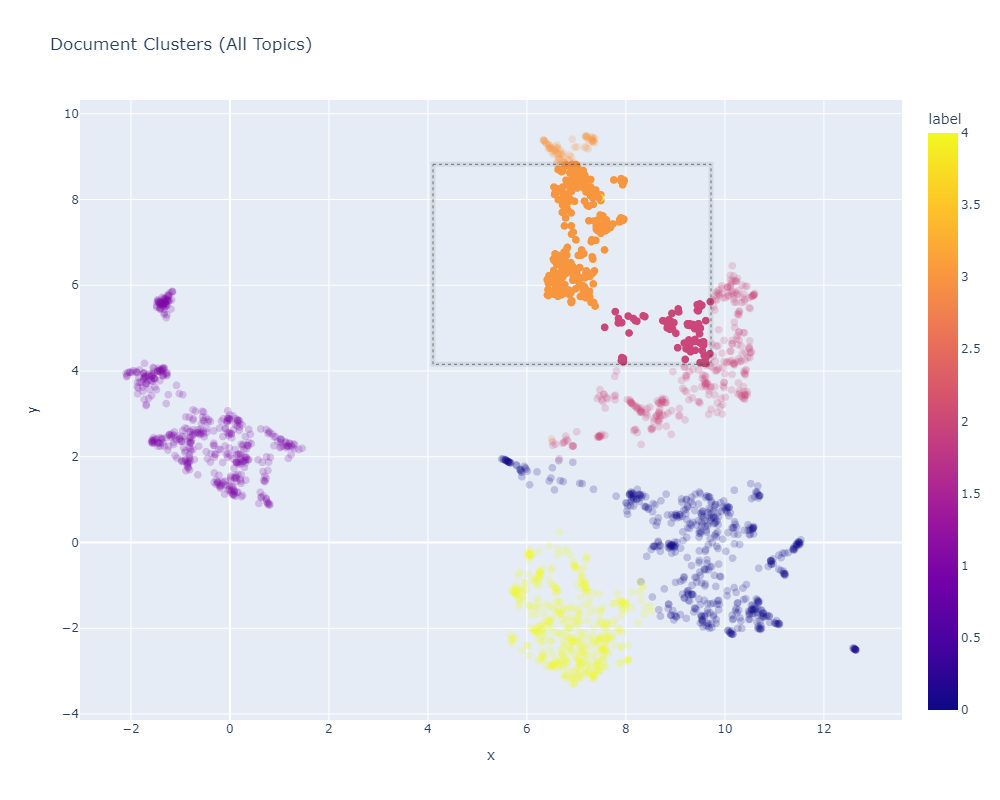
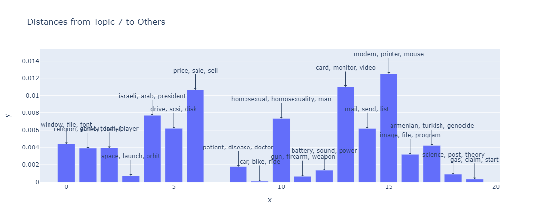
Visualize the results:

from stream.visuals import visualize_topic_model, visualize_topics

visualize_topic_model(
    model, 
    reduce_first=True, 
    port=8051,
    )

Downstream Tasks

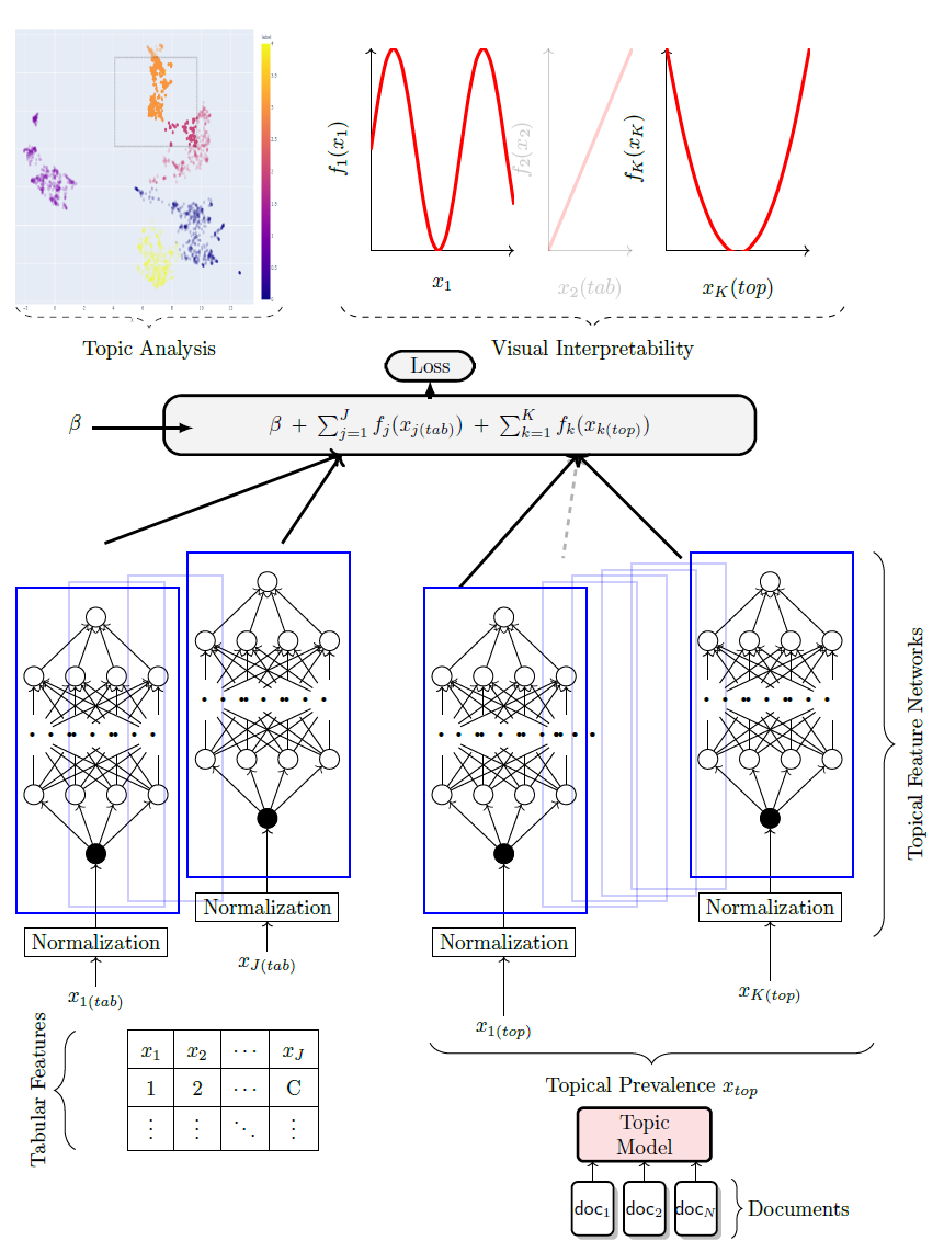
The general formulation of a Neural Additive Model (NAM) can be summarized by the equation:

$$ E(y) = h(β + ∑_{j=1}^{J} f_j(x_j)), $$

where $h(·)$ denotes the activation function in the output layer, such as a linear activation for regression tasks or softmax for classification tasks. $x ∈ R^j$ represents the input features, and $β$ is the intercept. The function $f_j : R → R$ corresponds to the Multi-Layer Perceptron (MLP) for the $j$-th feature.

Let's consider $x$ as a combination of categorical and numerical features $x_{tab}$ and document features $x_{doc}$. After applying a topic model, STREAM extracts topical prevalences from documents, effectively transforming the input into $z ≡ (x_{tab}, x_{top})$, a probability vector over documents and topics. Here, $x_{j(tab)}^{(i)}$ indicates the $j$-th tabular feature of the $i$-th observation, and $x_{k(top)}^{(i)}$ represents the $i$-th document's topical prevalence for topic $k$.

For preserving interpretability, the downstream model is defined as:

$$ h(E[y]) = β + ∑_{j=1}^{J} f_j(x_{j(tab)}) + ∑_{k=1}^{K} f_k(x_{k(top)}), $$

In this setup, visualizing the shape function k reveals the impact of a topic on the target variable y. For example, in the context of the Spotify dataset, this could illustrate how a topic influences a song's popularity.

Fitting a downstream model with a pre-trained topic model is straightforward using the PyTorch Trainer class. Subsequently, visualizing all shape functions can be done similarly to the approach described by Agarwal et al. (2021).

Python Example

from pytorch_lightning import Trainer
from stream.NAM import DownstreamModel

# Instantiate the DownstreamModel
downstream_model = DownstreamModel(
    trained_topic_model=topic_model,
    target_column='popularity',  # Target variable
    task='regression',  # or 'classification'
    dataset=dataset,  
    batch_size=128,
    lr=0.0005
)

# Use PyTorch Lightning's Trainer to train and validate the model
trainer = Trainer(max_epochs=10)
trainer.fit(downstream_model)

# Plotting
from stream.visuals import plot_downstream_model
plot_downstream_model(downstream_model)

ChrisW09/STREAM