Christian Ayala
This repository intendts to serve as a guide on how to analyze Feature
abundance and annotation data generated with the Compound Discoverer
software. The idea is to expand and customize the analysis and figures
that can be generated directly with Compound Discoverer to allow for
more detailed or in-depth analysis of the data. All the code and data
mentioned in this tutorial can be found in the file
c_disc_analysis.Rmd of this repository.
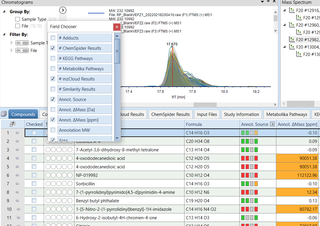
In the Compounds tab of Compound Discoverer results visualization select the following Field to export:
- Annot. $\Delta$Mass [ppm]
- Area
- Calc. MW
- Formula
- Gap Status
- Gap Fill Status
- MS2
- Name
- RT [min]
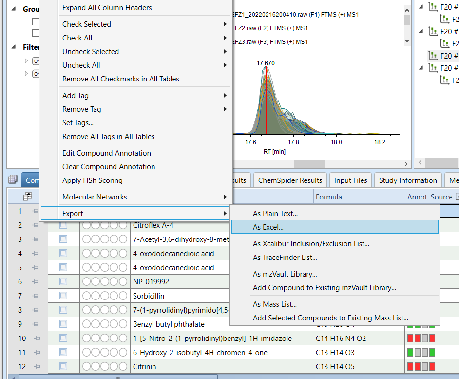
Then, right-click on the headers and select Export -> As Excel
Save the exported data in the inputs directory.
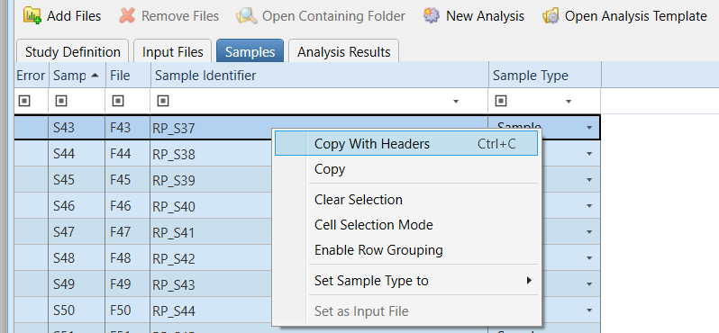
A metadata file with information about the samples (i.e., treatment, experimental conditions) is needed for the analysis. This file can be created by selecting and copying all rows of the Sample information table in the Samples tab of the Compound Discoverer Study files (see picture below), or can be created manually.
This repository can be clone to quickly download the R MarkDown script
(c_disc_analysis.Rmd), the custom functions and the tutorial data.
git clone https://github.com/Coayala/c_discoverer_data_analysis_tutorial.git
It is good practice to create an individual R project for each data
set that is going to be analyzed. Creating and R project which also
allow the library here used in this tutorial to work properly for path
set up.
To analyze the data generated by Compound Discoverer the following libraries are needed
library(tidyverse)
library(readxl)
library(ggpubr)
library(ggsci)
library(vegan)
library(rstatix)
library(factoextra)
library(ComplexHeatmap)
library(here)The following files provide a set of custom functions to quickly analyze the data
source('custom_functions/functions_cdis_exploration.R')
source('custom_functions/functions_cdis_norm_stats.R')
source('custom_functions/functions_cdis_diff.R')In this section we will set up variables that will be sued throughout the script. This includes create directories to contain the outputs (i.e., figures and tables) that will be generated with this script.
Setting up directory paths
# Main results folder
project_dir <- here('cd_tutorial_results')

# Figures output directory
figures_dir <- here(project_dir, 'figures')

# Tables output directory
tables_dir <- here(project_dir, 'tables')
Creating directories
To create the directories use the function walk to repeat the same
function over a list of variables. Throughout this script the iteration
functions from the purrr package (e.g., map and walk) will be
used. To learn more about iterations using purrr please check
here
dirs <- c(project_dir, figures_dir, tables_dir)
walk(dirs, function(x){
  if(!dir.exists(x)) dir.create(x)
})
Creating a theme
A object with theme options that will be used for all of th figures will be created to avoid repeating lines of code.
my_theme <- theme_bw() +
  theme(plot.title = element_text(face = 'bold', hjust = 0.5),
        axis.title = element_text(face = 'bold', hjust = 0.5),
axis.text.x = element_text(angle = 45, hjust = 1))Opening and rearranging the exported feature data table.
In this step a unique identifier (FeatureID) will be assigned to each
detected peak. Additionally, the annotation of compounds with and error
of mutate call.
cd_results_table <- read_xlsx(here('inputs', 'feature_data.xlsx')) %>%
  # Removing annotations of peaks with high ppm errors
  mutate(Name = ifelse(abs(`Annot. DeltaMass [ppm]`) > 5, NA, Name),
         Formula = ifelse(abs(`Annot. DeltaMass [ppm]`) > 5, NA, Formula)) %>%
  arrange(desc(`Calc. MW`)) %>%
  mutate(FeatureID = paste0('Feature',formatC(n():0001,
                                              width = 4,
                                              flag = '0'))) %>%
  select(FeatureID, Name, Formula, `Calc. MW`,
         contains('Annotation source'), contains('Results'),
         contains('Pathways'),
         contains('Area:'),
         contains('Gap Status:'),
         contains('Gap Fill Status:')) %>%
  # Differentiate between features that share the same name using "peak#" at the end of the name
  group_by(Name) %>%
  add_count(Name) %>%
  # Create variable with names for plotting (useful in following scripts)
  mutate(name4plot = case_when(is.na(Name) ~ FeatureID,
                               n == 1 ~ Name,
                               TRUE ~  paste0(Name, '-peak', n():1))) %>%
  select(-n) %>%
  ungroup()
Opening metadata file
metadata <- read_csv(here('inputs', 'metadata.csv'))## Rows: 72 Columns: 4
## ── Column specification ────────────────────────────────────────────────────────
## Delimiter: ","
## chr (4): SampleID, soil, treatment, time
##
## ℹ Use `spec()` to retrieve the full column specification for this data.
## ℹ Specify the column types or set `show_col_types = FALSE` to quiet this message.
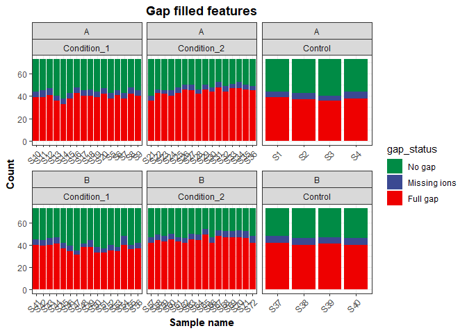
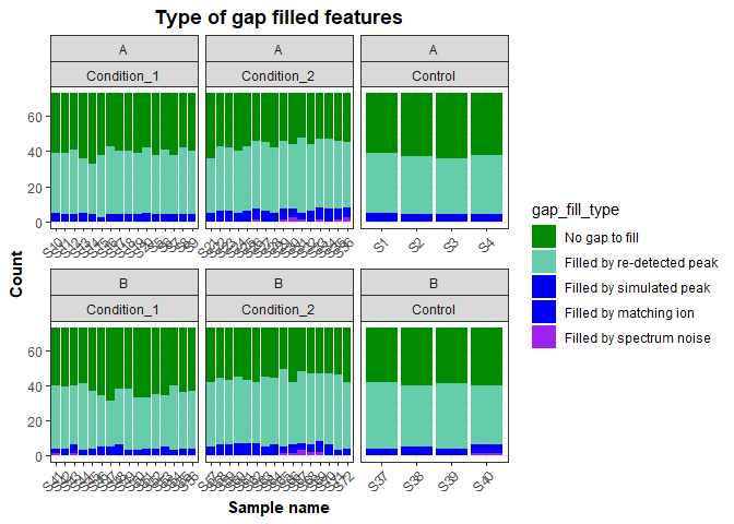
Check how many of the features were gap-filled to determine if the parameters on Compound Discoverer were good, or if they need to be changed.
Number of gap filled features per sample
Calculating the number of gap filled features based on the Gap Status columns from C. Discoverer results
gap_status <- cd_results_table %>%
  select(FeatureID, contains('Gap Status:')) %>%
  pivot_longer(contains('Gap Status:'), names_to = 'SampleID', values_to = 'gap_status') %>%
  mutate(SampleID = str_remove(SampleID, 'Gap Status: '),
         SampleID = str_remove(SampleID, '.raw.*'),
         gap_status = factor(gap_status, levels = c('No gap', 'Missing ions', 'Full gap')))
To plot the result, first we count how many times each gap status appears per sample.
gap_status_plot <- gap_status %>%
  group_by(SampleID) %>%
  count(gap_status) %>%
  left_join(metadata, by = 'SampleID') %>%
  ggplot() +
  geom_col(aes(x = SampleID,
               y = n,
               fill = gap_status)) +
  facet_wrap(~ soil + treatment, scales = 'free_x') +
  scale_fill_manual(values = c('#008B45FF', '#3B4992FF', '#EE0000FF')) +
  labs(x = 'Sample name',
       y = 'Count',
       title = 'Gap filled features') +
  my_theme

gap_status_plot
Gap filling methods per sample
If more detailed information about how data was gap filled we can use the Gap Fill Status columns from C. Discoverer. The type of gap filling was obtained by comparing the numbers in the Excel file, to the information that appear when hovering over C. Discoverer results.
gap_fill_status <- cd_results_table%>%
  select(FeatureID, Name, contains('Gap Fill Status:')) %>%
  pivot_longer(contains('Gap Fill Status:'), names_to = 'SampleID', values_to = 'gap_fill') %>%
  mutate(SampleID = str_remove(SampleID, 'Gap Fill Status: '),
         SampleID = str_remove(SampleID, '.raw.*')) %>%
  mutate(gap_fill_type = case_when(gap_fill == 32 ~ 'Filled by spectrum noise',
                                   gap_fill == 128 ~ 'Filled by re-detected peak',
                                   gap_fill == 0 ~ 'No gap to fill',
                                   gap_fill == 16 ~ 'Filled by simulated peak',
                                   gap_fill == 8 ~ 'Filled by trace area',
                                   gap_fill == 64 ~ 'Filled by matching ion')) %>%
  mutate(gap_fill_type = factor(gap_fill_type,
                                levels = c('No gap to fill', 'Filled by re-detected peak',
                                           'Filled by simulated peak', 'Filled by matching ion',
                                           'Filled by trace area', 'Filled by spectrum noise')))
Plotting the results
gap_summary_plot <-  gap_fill_status %>%
  select(SampleID, gap_fill_type) %>%
  group_by(SampleID) %>%
  count(gap_fill_type) %>%
  left_join(metadata, by = 'SampleID') %>%
   ggplot() +
  geom_col(aes(x = SampleID,
               y = n,
               fill = gap_fill_type)) +
  facet_wrap(~ soil + treatment, scales = 'free_x') +
  scale_fill_manual(values = c('green4', 'aquamarine3', 'blue2', 'blue', 'purple', 'firebrick2')) +
  labs(x = 'Sample name',
       y = 'Count',
       title = 'Type of gap filled features') +
  my_theme


gap_summary_plotThe custom functions in the functions_cdis_exploration.R file are used
to rearrange the data and calculate biochemical indexes (useful to
compare samples when there is not enough annotation). The biochemical
indexes are calculated with the same formulas used in
MetaboDirect.
# Split formula column into elemental counts
cd_results_table <- separate_formula(cd_results_table) %>%
  # Calculate ratios and thermodynamic indices
  calc_ratios_n_idxs(.)
## Joining, by = c("FeatureID", "Formula")
## Joining, by = c("FeatureID", "Formula")
## Joining, by = c("FeatureID", "Formula")
## Joining, by = c("FeatureID", "Formula")
## Joining, by = c("FeatureID", "Formula")
## Joining, by = c("FeatureID", "Formula")
Compounds can be classified in putative molecular classes based on their molecular formula. This not a completely accurate classification for LC-MS/MS data, if you InChIKeys or InCHI for your features please use Classyfire instead.
cd_results_table <- calc_classes(cd_results_table)compounds_table <- cd_results_table %>%
select(-contains('Gap Status:'), -contains('Labeling Status:'), -contains('Gap Fill Status:')) %>%
pivot_longer(contains('Area:'), names_to = 'SampleID', values_to = 'AUC') %>%
mutate(SampleID = str_remove(SampleID, 'Area: '),
SampleID = str_remove(SampleID, '.raw.*')) %>%
left_join(metadata, by = 'SampleID')
auc_matrix <- compounds_table %>%
select(FeatureID, SampleID, AUC) %>%
pivot_wider(names_from = 'SampleID', values_from = 'AUC') %>%
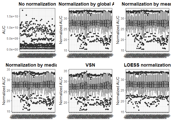
column_to_rownames(var = 'FeatureID')Several data normalization methods can be applied. To test a few of them we can use custom functions
normalize_by_all(auc_matrix)The best normalization method appears to be LOESS normalization. That
is the one that will be used for the next steps
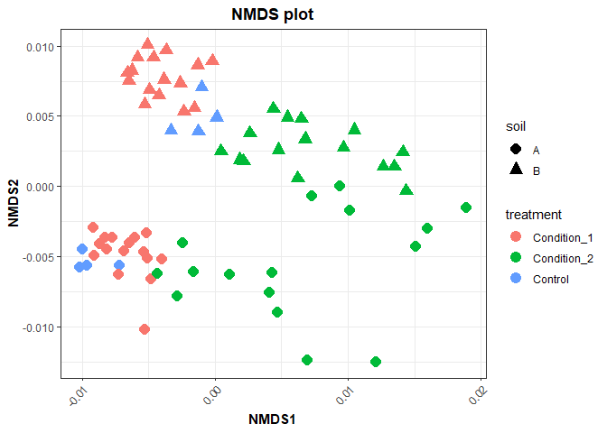
norm_matrix <- cycloess.norm(auc_matrix)NMDS is an ordination method that can use different distance matrices to
cluster the data. For this particular dataset, since we have relative
abundances we are using bray_curtis distances.
Calculating distance matrix
# distance matrix by Bray because relative abundance mode was selected
dm <- t(norm_matrix) %>%
  vegdist(., method = 'bray')
Performing NMDS analysis
nmds_res <- metaMDS(dm,
          k = 2,
          maxit = 999,
          trymax = 500,
          wascores = TRUE)
## Run 0 stress 0.1220264
## Run 1 stress 0.1220264
## ... Procrustes: rmse 1.610821e-05 max resid 0.0001115948
## ... Similar to previous best
## Run 2 stress 0.1222021
## ... Procrustes: rmse 0.008394484 max resid 0.05146383
## Run 3 stress 0.2464701
## Run 4 stress 0.1219992
## ... New best solution
## ... Procrustes: rmse 0.006516641 max resid 0.05233997
## Run 5 stress 0.1219992
## ... Procrustes: rmse 1.134487e-05 max resid 8.358761e-05
## ... Similar to previous best
## Run 6 stress 0.1220264
## ... Procrustes: rmse 0.00651646 max resid 0.05230921
## Run 7 stress 0.1222021
## ... Procrustes: rmse 0.005683796 max resid 0.04497399
## Run 8 stress 0.1221682
## ... Procrustes: rmse 0.009325697 max resid 0.05263667
## Run 9 stress 0.1222021
## ... Procrustes: rmse 0.005676546 max resid 0.04491296
## Run 10 stress 0.1221628
## ... Procrustes: rmse 0.009024195 max resid 0.05247348
## Run 11 stress 0.1221682
## ... Procrustes: rmse 0.009307805 max resid 0.05263368
## Run 12 stress 0.2500392
## Run 13 stress 0.1221682
## ... Procrustes: rmse 0.009324797 max resid 0.05263568
## Run 14 stress 0.1220264
## ... Procrustes: rmse 0.006515991 max resid 0.05231059
## Run 15 stress 0.1221682
## ... Procrustes: rmse 0.009312747 max resid 0.05263706
## Run 16 stress 0.1221628
## ... Procrustes: rmse 0.009035963 max resid 0.05247377
## Run 17 stress 0.1220264
## ... Procrustes: rmse 0.006515852 max resid 0.05230882
## Run 18 stress 0.1222022
## ... Procrustes: rmse 0.005612371 max resid 0.04437781
## Run 19 stress 0.1220264
## ... Procrustes: rmse 0.006515756 max resid 0.0523089
## Run 20 stress 0.1220264
## ... Procrustes: rmse 0.006516421 max resid 0.0523094
## *** Solution reached
Extracting NMDS scores and plotting
nmds_scores <- as.data.frame(scores(nmds_res, display = 'sites')) %>%
    rownames_to_column(var = 'SampleID') %>%
    left_join(metadata, by = 'SampleID')


nmds_plot <- nmds_scores %>%
    ggplot() +
    geom_point(aes(x = NMDS1,
                   y = NMDS2,
                   color = treatment,
                   shape = soil),
               size = 4) +
    labs(title = 'NMDS plot') +
    my_theme

nmds_plot