Geographic-Information-Systems-and-Science-assessment-

中文版会在我写完之后发布，现在只有英文版. 请勿转载，谢谢 This tutorial is fully made by author, do not reprint without permit This tutorial aims to use GWR to find the coefficients of influcing factors of window opening in China. It has been divided into these parts : Bubble map, OLS model, Moran's I, GWR

Bubble map

The bubble map code in R is shown in the bellow:

library(ggplot2)
library(ggmap)
library(maptools)
library(maps)
library(dplyr)
library(viridis)
library(mapproj)
library(readr)

China <- map_data("world") %>% filter(region=="China") #Region of China
myData <- read.csv('cw/ex.csv') # Read file
myBreaks <- c(0.1,0.3, 0.5,0.7, 1)

# Plot map
map <- 
  ggplot() +
  geom_polygon(data=China,aes(long, y = lat, group = group), fill="white", alpha=0.3) +
  geom_point(data=myData, aes(x=longitude, y = latitude, size=open.rate, color=open.rate, alpha=open.rate), shape=20, stroke=FALSE) +
  scale_size_continuous(name="Opening rate", trans="sqrt", range=c(1,12), breaks=myBreaks) +
  scale_alpha_continuous(name="Opening rate", trans="sqrt", range=c(0.1, 0.6), breaks=myBreaks) +
  scale_color_viridis(option="magma", trans="sqrt", breaks=myBreaks, name="Opening rate" ) + #Transformation "sqrt"
  theme_void()  + coord_map() +  xlim(70,149)+ ylim(18,55)+
  guides( colour = guide_legend()) +
  ggtitle("Window opening rate in China") +
  theme(
    legend.position = c(0.85, 0.8),
    text = element_text(color = "#f5f5f2"), # Choose colour
    plot.background = element_rect(fill = "#4e4d47", color = NA), 
    panel.background = element_rect(fill = "#4e4d47", color = NA), 
    legend.background = element_rect(fill = "#4e4d47", color = NA),
    plot.title = element_text(size= 16, hjust=0.1, color = "#f5f5f2", margin = margin(b = -0.1, t = 0.4, l = 2, unit = "cm")),
  )
plot(map)

The result of the data distribution. The dataset consists of 95 cities with window opening rate (dependent variable), and four other variables.

OLS model

First the library in R we need:

library(tmap)
library(readr)
library(rgdal)
library(ggplot2)
library(ggmap)
library(maptools)
library(maps)
library(dplyr)
library(viridis)
library(mapproj)
library(spdep)
library(car)
library(spgwr)

If you need to download the shapefile of China, you can find from here. First let's look at the OLS model:

chinaSHP <- readOGR("exe/gadm36_CHN_1.shp")# Read SHP file
dataWindow <- read_csv("cw/data.csv") # Read data
model <- lm(`open rate` ~ `Dry-bulb temperature`+`Wind speed`+`External relative humidity`
            +`Atmospheric pressure`,data=dataWindow) # OLS model
summary(model)
plot(model) # Plot result
durbinWatsonTest(model) #Autocorrelation

lm(formula = `open rate` ~ `Dry-bulb temperature` + `Wind speed` + 
    `External relative humidity` + `Atmospheric pressure`, data = dataWindow)

Residuals:
      Min        1Q    Median        3Q       Max 
-0.153347 -0.035615  0.009812  0.031448  0.251990 

Coefficients:
                               Estimate Std. Error t value Pr(>|t|)    
(Intercept)                  -0.2491505  0.0600809  -4.147 7.62e-05 ***
`Dry-bulb temperature`        0.0569267  0.0024493  23.242  < 2e-16 ***
`Wind speed`                  0.0036693  0.0069773   0.526  0.60026    
`External relative humidity`  0.0005466  0.0005036   1.085  0.28060    
`Atmospheric pressure`       -0.0027743  0.0008336  -3.328  0.00127 ** 
---
Signif. codes:  0 ‘***’ 0.001 ‘**’ 0.01 ‘*’ 0.05 ‘.’ 0.1 ‘ ’ 1

Residual standard error: 0.06105 on 90 degrees of freedom
Multiple R-squared:  0.8957,	Adjusted R-squared:  0.8911 
F-statistic: 193.3 on 4 and 90 DF,  p-value: < 2.2e-16

It can be seen that some variable (wind speed,humidity) is not significant,the p-value is higher than 0.05. However, these variable is kept because these variable may not significant in overall model, but significant in each local model in GWR.

 lag Autocorrelation D-W Statistic p-value
   1      0.06111587      1.846829   0.376
 Alternative hypothesis: rho != 0

DW statistics for our model is 1.84, it seems that it shoud be fine. However!!!! WE ARE USING GWR Thus, there may have spatial-autocorrelation. Let's have a look:

dataWindow$residuals <- residuals(model) 

#Function to plot residuals
bubblefunc <- function(myData,size,name,myBreaks){
  China <- map_data("world") %>% filter(region=="China")
  map <- 
    ggplot() +
    geom_polygon(data=China,aes(long, y = lat, group = group), fill="white", alpha=0.3) +
    geom_point(data=myData, aes(x=longitude, y = latitude, size=size, color=size, alpha=size), shape=20, stroke=FALSE) +
    scale_size_continuous(name=name,  trans="identity",range=c(1,12),breaks=myBreaks) +
    scale_alpha_continuous(name=name, trans="identity", range=c(0.1, 0.6),breaks=myBreaks) +
    scale_color_viridis(option="magma", trans="identity", name=name,breaks=myBreaks ) + 
    theme_void()  + coord_map() +  xlim(70,149)+ ylim(18,55)+
    guides( colour = guide_legend()) +
    ggtitle(paste("Window opening rate" ,name,"in China")) +
    theme(
      legend.position = c(0.85, 0.8),
      text = element_text(color = "#f5f5f2",size=15), # Choose colour
      plot.background = element_rect(fill = "#4e4d47", color = NA), 
      panel.background = element_rect(fill = "#4e4d47", color = NA), 
      legend.background = element_rect(fill = "#4e4d47", color = NA),
      plot.title = element_text(size= 16, hjust=0.1, color = "#f5f5f2", margin = margin(b = -0.1, t = 0.4, l = 2, unit = "cm")),
    )
  plot(map)
}
bubblefunc(dataWindow,dataWindow$residuals,"Residuals",c(-0.2,-0.1,0,0.1,0.3)) # Plot residuals

The south part of China has higher residual and the pink areas are close to other pink areas. In other words, we may have some spatial autocorrelation. Let's use moran's I to test more systematically.

Moran's I

xy=dataWindow[,c(13,14)]
chinasf <- st_as_sf(x=xy,coords = c("longitude", "latitude"))
chinasp <- as(chinasf, "Spatial") # Transform to "spatial"

coordsW <- coordinates(chinasp) # calculate the centroids of all Wards in London
plot(coordsW)
knn_wards <- knearneigh(coordsW, k=4)# nearest neighbours
LWard_knn <- knn2nb(knn_wards)
plot(LWard_knn, coordinates(coordsW), col="blue") #Plot
#create a spatial weights matrix object from  weight
Lward.knn_4_weight <- nb2listw(LWard_knn, style="C")
#moran's I test on the residuals
moran.test(dataWindow$residuals, Lward.knn_4_weight)

	Moran I test under randomisation

data:  dataWindow$residuals  
weights: Lward.knn_4_weight    

Moran I statistic standard deviate = 2.7069, p-value = 0.003396
alternative hypothesis: greater
sample estimates:
Moran I statistic       Expectation          Variance 
      0.166649889      -0.010638298       0.004289717

Moran I is within range of -1 to 1, and 0 means no spatial autocorrelation. Here, Moran's I is 0.167, which implies that we may have some weak spatial autocorrelation in our residuals. Therefore, GWR is used to address this problem.

GWR model

#calculate kernel bandwidth
GWRbandwidth <- gwr.sel(`open rate` ~ `Dry-bulb temperature`+`Wind speed`+`External relative humidity`
                     +`Atmospheric pressure`,data=dataWindow,coords=coordsW,adapt=T)
#run the gwr model
GWRModel <- gwr(`open rate` ~ `Dry-bulb temperature`+`Wind speed`+`External relative humidity`
                +`Atmospheric pressure`,data=dataWindow,coords=coordsW,adapt=GWRbandwidth,
                hatmatrix = TRUE,se.fit = TRUE)
GWRModel #print the results of the model
results<-as.data.frame(GWRModel$SDF)
names(results)

gwr(formula = `open rate` ~ `Dry-bulb temperature` + 
    `Wind speed` + `External relative humidity` + 
    `Atmospheric pressure`, data = dataWindow, coords = coordsW, 
    adapt = GWRbandwidth, hatmatrix = TRUE, se.fit = TRUE)
Kernel function: gwr.Gauss 
Adaptive quantile: 0.0333945 (about 3 of 95 data points)
Summary of GWR coefficient estimates at data points:
                                     Min.     1st Qu.      Median     3rd Qu.        Max.  Global
X.Intercept.                  -1.55295044 -0.56679395 -0.30426784 -0.12435906  0.40684111 -0.2492
X.Dry.bulb.temperature.        0.02109119  0.05192010  0.06482929  0.06990573  0.08456590  0.0569
X.Wind.speed.                 -0.09409310 -0.00837505 -0.00171803  0.00572094  0.02819445  0.0037
X.External.relative.humidity. -0.00539565 -0.00085167  0.00093522  0.00260762  0.01414508  0.0005
X.Atmospheric.pressure.       -0.02081367 -0.00529484 -0.00299928  0.00036854  0.01054743 -0.0028
Number of data points: 95 
Effective number of parameters (residual: 2traceS - traceS'S): 55.28598 
Effective degrees of freedom (residual: 2traceS - traceS'S): 39.71402 
Sigma (residual: 2traceS - traceS'S): 0.03666693 
Effective number of parameters (model: traceS): 44.0667 
Effective degrees of freedom (model: traceS): 50.9333 
Sigma (model: traceS): 0.03237767 
Sigma (ML): 0.02370744 
AICc (GWR p. 61, eq 2.33; p. 96, eq. 4.21): -266.3886 
AIC (GWR p. 96, eq. 4.22): -397.3086 
Residual sum of squares: 0.05339408 
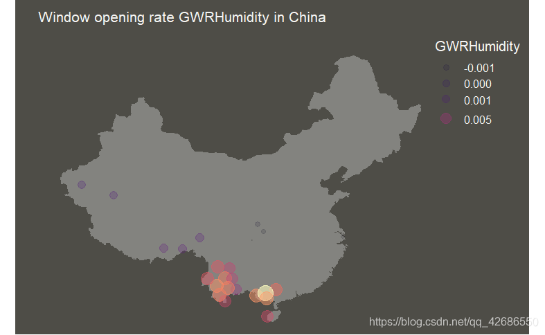
Quasi-global R2: 0.9834058

It can be seen that the value of coefficient of each variable is different in each localation. sometimes it's positive and sometimes it's negative. Let's make a map for temperature this variable:

dataWindow$coeTemperature <- results$X.Dry.bulb.temperature.
bubblefunc(dataWindow,dataWindow$coeTemperature,'coeTemperature',c(0.02,0.05, 0.06,0.07, 0.08))

The south part of region has higher coefficient than other areas. However, we still need to take significance into account. In this study, if a coefficient estimate is more than 2 standard errors away from zero, then it is “statistically significant”.

#statistically significant test
sigTest_Temp = abs(GWRModel$SDF$"`Dry-bulb temperature`") - 2 * GWRModel$SDF$"`Dry-bulb temperature`_se"
dataWindow$GWRTemp <- sigTest_Temp
bubblefunc(subset(dataWindow,dataWindow$GWRTemp>0),subset(dataWindow$coeTemperature,dataWindow$GWRTemp>0),'GWRTemp ',c(0.02,0.05, 0.06,0.07, 0.08))

A lot of varables in temperature seems signficant. Similary, let's look at other varables: It can be seen that the coefficient have significant different in other varibales. Therefore, the influencing factors of window have spatial variations.

Connor666/Geographic-Information-Systems-and-Science-assessment

Geographic-Information-Systems-and-Science-assessment-

Bubble map

OLS model

Moran's I

GWR model