You can use this file as a template for your writeup if you want to submit it as a markdown file, but feel free to use some other method and submit a pdf if you prefer.
Advanced Lane Finding Project
The goals / steps of this project are the following:
- Compute the camera calibration matrix and distortion coefficients given a set of chessboard images.
- Apply a distortion correction to raw images.
- Use color transforms, gradients, etc., to create a thresholded binary image.
- Apply a perspective transform to rectify binary image ("birds-eye view").
- Detect lane pixels and fit to find the lane boundary.
- Determine the curvature of the lane and vehicle position with respect to center.
- Warp the detected lane boundaries back onto the original image.
- Output visual display of the lane boundaries and numerical estimation of lane curvature and vehicle position.
Rubric Points
Here I will consider the rubric points individually and describe how I addressed each point in my implementation.
1. Provide a Writeup / README that includes all the rubric points and how you addressed each one. You can submit your writeup as markdown or pdf. Here is a template writeup for this project you can use as a guide and a starting point.
You're reading it!
All code for the following steps and images/videos are contained in the code cells of the Jupyter notebook located in "./AdvancedLaneDetection.ipynb".
1. Briefly state how you computed the camera matrix and distortion coefficients. Provide an example of a distortion corrected calibration image.
Refer to code cell #1.
I start by preparing "object points", which will be the (x, y, z) coordinates of the chessboard corners in the world. Here I am assuming the chessboard is fixed on the (x, y) plane at z=0, such that the object points are the same for each calibration image. Thus, objp is just a replicated array of coordinates, and objpoints will be appended with a copy of it every time I successfully detect all chessboard corners in a test image. imgpoints will be appended with the (x, y) pixel position of each of the corners in the image plane with each successful chessboard detection.
I then used the output objpoints and imgpoints to compute the camera calibration and distortion coefficients using the cv2.calibrateCamera() function. I applied this distortion correction to the test image using the cv2.undistort() function as well as the perspective transform warp cv2.warpPerspective and obtained this result:
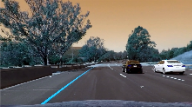
To demonstrate this step, I will describe how I apply the distortion correction to one of the test images like this one:

I simply save the calibrated camera and undistort the given images using the following function:
def undistort(img, objpoints, imgpoints, mtx):
    gray = cv2.cvtColor(img,cv2.COLOR_BGR2GRAY)
    ret, mtx, dist, rvecs, tvecs = cv2.calibrateCamera(objpoints, imgpoints, gray.shape[::-1], mtx, None)
    undist = cv2.undistort(img, mtx, dist, None, mtx)
    return undist
2. Describe how (and identify where in your code) you used color transforms, gradients or other methods to create a thresholded binary image. Provide an example of a binary image result.
Refer to code cell #3.
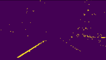
I used a combination of color and gradient thresholds to generate a binary image. In particular, I used the function color_xgrad_bin_pipeline with the thresholds of xgrad_thresh=(15, 25) and s_thresh=(170,200) for most of the pipelines. Here's an example of my output for this step.
3. Describe how (and identify where in your code) you performed a perspective transform and provide an example of a transformed image.
Refer to code cells #4 (warper) and #5 (show_lanes_superimposed).
The code for my perspective transform includes a function called warper(). The warper() function takes as inputs an image (img), as well as source (src) and destination (dst) points. I chose the hardcode the source and destination points in the following manner:
src = np.float32(
    [[(img_size[0] / 2) - 55, img_size[1] / 2 + 100],
    [((img_size[0] / 6) - 10), img_size[1]],
    [(img_size[0] * 5 / 6) + 60, img_size[1]],
    [(img_size[0] / 2 + 55), img_size[1] / 2 + 100]])
dst = np.float32(
    [[(img_size[0] / 4), 0],
    [(img_size[0] / 4), img_size[1]],
    [(img_size[0] * 3 / 4), img_size[1]],
    [(img_size[0] * 3 / 4), 0]])
This resulted in the following source and destination points:
| Source | Destination |
|---|---|
| 585, 460 | 320, 0 |
| 203, 720 | 320, 720 |
| 1127, 720 | 960, 720 |
| 695, 460 | 960, 0 |
I verified that my perspective transform was working as expected (show_lanes_superimposed) by drawing the src and dst points onto a test image and its warped counterpart to verify that the lines appear parallel in the warped image.
4. Describe how (and identify where in your code) you identified lane-line pixels and fit their positions with a polynomial?
Refer to code cell #5.
Using the color/gradient-thresholded warped perspectives and the histogram of detected points for that image, I detected the points that would comprise the line via a sliding window of reasonably-bounded rectangles, totalling 9 windows. After saving the associated x and y points for each detected lane, I fit my lane lines with a 2nd order polynomial kinda like this:
5. Describe how (and identify where in your code) you calculated the radius of curvature of the lane and the position of the vehicle with respect to center.
Refer to code cell #5 (calculate_stats).
Using the given example again, I used the max y-coordinates (lowest in image) as an initial anchor for the pixel-based curvature radii. This was followed by computing the meters curvature radii via the conversion:
ym_per_pix = 30/720 # meters per pixel in y dimension
xm_per_pix = 3.7/700 # meters per pixel in x dimension

# Fit new polynomials to x,y in world space
left_fit_cr = np.polyfit(lefty*ym_per_pix, leftx*xm_per_pix, 2)
right_fit_cr = np.polyfit(righty*ym_per_pix, rightx*xm_per_pix, 2)
# Calculate the new radii of curvature
left_curve_radius = ((1 + (2*left_fit_cr[0]*left_y_eval*ym_per_pix + left_fit_cr[1])**2)**1.5) / np.absolute(2*left_fit_cr[0])
right_curve_radius = ((1 + (2*right_fit_cr[0]*right_y_eval*ym_per_pix + right_fit_cr[1])**2)**1.5) / np.absolute(2*right_fit_cr[0])
The overall cuvature radius was calculated by averaging the two lane curvature radii:
curvature = (left_curve_radius + right_curve_radius) / 2.
Inspired by https://github.com/sumitborar/AdvancedLaneDetection/blob/master/Advanced%20Lane%20Detection.ipynb, I added an extra sanity check by calculating the left curvature radius to right curvature radius ratio:
ratio = left_curve_radius / right_curve_radius.
The current position of the vehicle in relation to the center of the lane is given by:
car_pos = ((img.shape[1] / 2) - ((lane_leftx + lane_rightx) / 2)) * xm_per_pix,
where (img.shape[1] / 2) is the image center, ((lane_leftx + lane_rightx) / 2) is the lane center, and the difference of the vehicle centering is converted from pixel space to meter space.
6. Provide an example image of your result plotted back down onto the road such that the lane area is identified clearly.
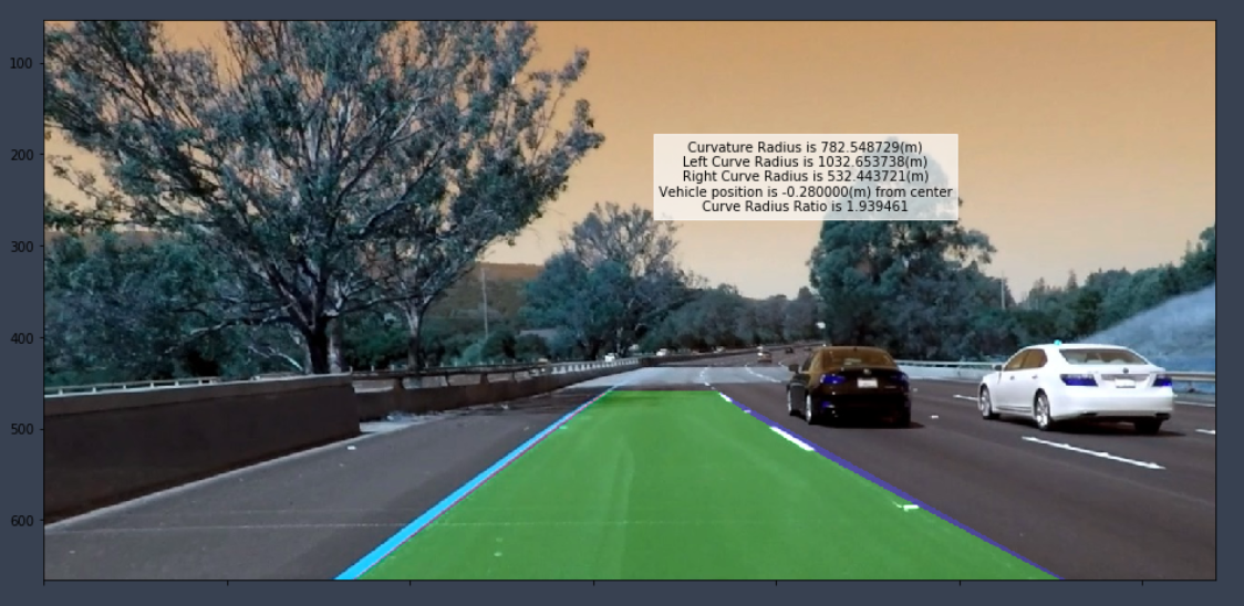
I implemented this step a few cells after finishing all of the components for a working pipeline. Please refer to code cell #9 (process_image) for a succinct pipeline on an image, which can be read and returned for a video. Here is an example of my result on a test image:
1. Provide a link to your final video output. Your pipeline should perform reasonably well on the entire project video (wobbly lines are ok but no catastrophic failures that would cause the car to drive off the road!).
Here's a link to my video result
1. Briefly discuss any problems / issues you faced in your implementation of this project. Where will your pipeline likely fail? What could you do to make it more robust?
Here I'll talk about the approach I took, what techniques I used, what worked and why, where the pipeline might fail and how I might improve it if I were going to pursue this project further.
Throughout the project, I was plagued with the reason why I do not have my laptop at the moment: my laptop would seemingly randomly restart. SMC crashes were found and the problem is being looked into.
Back to the project, most of the template routines were enough to tweek such that I could build an adequate pipeline from the pieces and accurately detect the lanes for the test images and video. I stayed with using the color/sobel-x gradient threshold since this was the simplest method to highlight the points in the image that I wanted. The thesholding here could certainly be tailored to better fit the data and a cool addition to this would be robustly come up with an ideal spectrum (white/yellow) for the lower half of the image. Something difficult in this is filtering out outliers (ie. a yellow piece of debris next to the lane boundary), which can be alleviated by the next steps. Drastic changes (especially within frame) in the lane curvature seemed to significantly confuse the lane detection pipeline. The first advancement that I will likely try is to incorporate the last n-1 lane 2-D polynomial fits and average them together. This should make the pipeline much more robust and smoothed over drastic turns in the road. Another problem that this would likely help with is elevation (not being able to see directly in front or a false assumption of flatness).


