Venus Lee and Jesse Wang
This is a repository for two mini machine learning projects using publically available battery data published by NASA at https://ti.arc.nasa.gov/tech/dash/groups/pcoe/prognostic-data-repository/#battery. Jump to the following sections to learn more:
This mini-project aims to develop a traditional machine learning model using scikit-learn to predict the current state of health (SoH) of a lithium ion battery, using voltage and temperature profiles from discharging cycles. In particular, we aim to predict the battery's remaining capacity in Ah, given data from any cycle. Our final model is a weighted voting ensemble incorporating random forest, extra trees, and XGBoost regressors, achieving a root mean squared error of 0.0160Ah on the test set.
- Create a new conda environment using
conda env create -f environment.yml. The first line of the.ymlfile sets the new environment's name (batteryenvby default). Activate the new environment usingconda activate batteryenv. - Run
model_building.ipynbto generate the ensemble voting regressorbest_voting.pkland the scalerscaler.pkllocally. - Run
python make_prediction.pyto randomly select a battery and cycle number, plot the associated voltage and temperature curves, and use our trained model to predict the capacity.
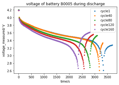
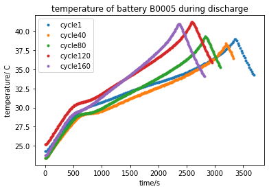
The experimental data consists of groups of experiments performed on Li-ion batteries with a rated capacity of 2Ah. In particular, batteries 5, 6, 7, and 18 were repeatedly charged to 4V and discharged at an ambient temperature of 24C, with a constant discharge current of 2A. The experiments on batteries 49, 50, 51, 53, 54, 55, and 56 were carried out at a temperature of 4C, using the same discharge current. The remaining capacities at each cycle were also recorded, in addition to the voltage and temperature profiles. We plot the voltage and temperature discharge profiles of battery #5 as an example below, for various cycle numbers:
We then extracted the following features from each cycle:
- Time taken for the discharging temperature to reach its maximum value
- Maximum temperature reached during discharge
- Average rate of temperature increase during discharge, as measured by (maximum temperature - initial temperature)/time taken
- Time for the measured voltage to drop below 3V
- Initial slope of the measured voltage
Initially we considered extracting features from the charging cycles as well; however the data was quite irregular and we determined that the effect on the final model could be ignored. A baseline random forest model indicates that the most important features are #4 (75% importance) and #1 (24% importance). Interestingly, the explicit dependence of ambient temperature of the experiment seems to be negligible.
After removing anomalies using isolation forest methods, we split the data (~1000 data points) into training, validation, and test sets in a 60:20:20 ratio. Each set was stratified according to the amount of cycle data available per battery. We then tried baseline models on default hyperparameters (random forest, extra trees, linear regression, elastic net regression, LGBM, XGBoost, SVM, and k-NN) using 5-fold cross validation on the train set and with RMSE as the evaluation metric. Further to this we selected the best three models - random forest, extra trees, and XGBoost - and performed hyperparameter tuning for each, evaluating the tuned models on the validation set to check for overfitting. Finally we combined the three tuned models into a voting ensemble, whose weights were optimized, and evaluated its performance on the test set.
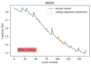
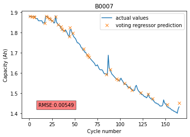
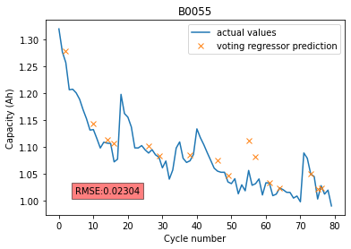
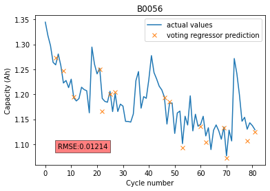
As our test set was stratified to include test examples of cycles from every battery, we can plot the actual measured capacities for each battery against our final model's predicted values for the chosen test examples. The results for a few selected batteries, and the associated errors, are shown below:
The overall RMSE achieved on the test set of 0.0160Ah is comparable to the error on the validation and training sets, which suggests that an appropriate amount of regularization has been applied to prevent overfitting.
In this mini-project, we train a sequence-to-sequence LSTM network in Keras to predict voltage discharging curves for the next 50 cycles, given 10 cycles' worth of data. The raw data consists of the voltage discharging curves from batteries 5, 6, and 7.
- Create a new conda environment using
conda env create -f environment.yml. The first line of the.ymlfile sets the new environment's name (batteryenvby default). Activate the new environment usingconda activate batteryenv. - Change the current directory using
cd discharge_curve_prediction. - Run
python display_results.py -b <battery_number> -s <starting_cycle>to use our trained model to make predictions and visualise them.<battery_number>is an integer from0to2, inclusive (0indicates battery B0005,1indicates battery B0006, and2indicates battery B0007).<starting_cycle>is an integer from0to107, inclusive. This refers to the first cycle from which data will be sampled.- For example, running
python display_results.py -b 1 -s 90will produce the following plots (note that only a subset of the green curves are shown):
B. Saha and K. Goebel (2007). "Battery Data Set", NASA Ames Prognostics Data Repository (http://ti.arc.nasa.gov/project/prognostic-data-repository), NASA Ames Research Center, Moffett Field, CA
