This github repo serves as the starting point for offline evaluation of submissions for the training data debugging vision benchmark. The offline evaluation can be run on both your local environment as well as a containerized image for reproducibility of score results.
For a detailed summary of the a benchmark, refer to the provided benchmark documentation.
A design document for the benchmark can be found here. Note that permission is required to view the benchmark design doc. Please join MLCommons/DataPerf Workgroup to request access or send an email to xiaozhe.yao@inf.ethz.ch
The following resources will need to be downloaded locally in order to run offline evaluation:
- Embeddings for candidate pool of training, validation and testing images (.parquet file)
- Ground truth labels for images (.csv files)
These resources can be downloaded in a .zip file at the following url
https://drive.google.com/file/d/1_-WZCGd31XTENCtVjP4GqDLYShP3NzwK/view?usp=sharing
For running as a containerized image:
dockerfor building the containerized imagedocker-composefor running the scoring service with the appropriate resources
Installation instructions can be found at the following links: Docker, Docker compose.
For running locally:
- Python (>= 3.7)
The current version of this repo has only been tested locally on Python 3.8 and Ubuntu 22.04.
Clone this repo to your local machine
$ git clone git@github.com:DS3Lab/dataperf-vision-debugging.git
If you want to run the offline evaluation in your local environment, install the required python packages
$ pip install -r requirements.txt
A template filesystem with the following structure is provided in the repo. By unzipping the resource file, the embeddings and ground truth will be placed in the appropriate folders.
$ unzip -o cleaning_challenge_data.zip
The resulting filesystem in the repo should look as follows
|____embeddings
| |____01g317_train_0.3_300.parquet
| |____01g317_test_500.parquet
With the resources in place, you can now test that the system is functioning as expected.
To test the containerized offline evaluation, run
$ docker-compose run dataperf-debugging-submissionSimilarly, to test the local python offline evaluation, run
$ python3 create_baselines.py && python3 main.py && python3 plotter.pyEither test will run the offline evaluation using the setup specified in task_setup.yaml (or task_setup_docker.yaml), which will utilise a training set (with some noise) and a validation set to generate baseline debugging strategies, train classification models and generate a plot in results/ with the data id.
|____results
| |____01g317_evaluation.png
For the alpha version of this benchmark we will only support submissions and offline evaluation for the open division.
A valid submission for the open division includes the following:
- A description of the data selection algorithm/strategy used
- A list of data points to be inspected and corrected
- (Optional) A script of the algorithm/strategy used
Each submission must be a .txt file. Each row in the file represents the index to the image label that needs to be inspected and corrected. The submission file should be named as {data_id}_{your_method_name}.txt, for example 01g317_random.txt or 01g317-flipped_neighbor_shapley.txt.
The included training set file serves as a template of a single submission:
$ head examples/01g317_my_method.txt

1
2
3
4
...
Besides of the data points to be inspected and corrected, the submission file also contains a text file that states how long your submission takes to get the submission file. This text file is used to compare your submission with the other submissions from the aspect of speed. The text file should be named as time_{data_id}_{your_method_name}.txt, for example time_01g317_random.txt. It should contain a single line with the time (in seconds) it takes to run the submission. For example,
$ head examples/time_01g317_my_method.txt

4.6976000021459186e-05
The configuration for the offline evaluation is specified in task_setup.yaml file (or task_setup_docker.yaml). For simplicity, the repo comes pre-configured such that for offline evaluation you can simply:
- Copy your training sets to the template filesystem
- Modify the config file to specify the training set for each task
- Run offline evaluation
- See results in stdout and results file in
results/
TBD.
TBD.
After running the evaluation, the results and figures are stored in results/. There will be one figure for each task, and an aggregated figure for all tasks.
Figure for Each Task
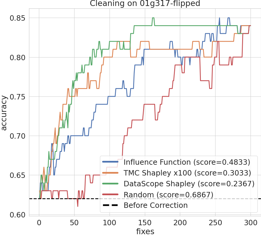
An example figure for a single task is shown below. The x-axis represents the number of data points each algorithm inspects, and the y-axis represents the test accuracy. The black dashed horizontal line represents the initial accuracy without any debugging. Intuitive, the higher the curve, the better the performance - meaning that the debugging algorithm leads to better performance with the same number of inspections.
Aggregated Figure
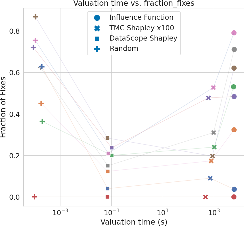
An example aggregated figure is shown below. This figure is used to compare different algorithms quantitatively. The x-axis represents the time each algorithm needs in order to find the order of debugging. Differernt shapes of marker indicates different tasks. The y-axis represents the portion of data points each algorithm needs to inspect, in order to achieve a high enough accuracy (95% of the accuracy on the cleaned training dataset). The y-axis represents the time each algorithm needs in order to find the order of debugging. Differernt shapes of marker indicates different tasks.
Intuitively, if the algorithm is higher, the algorithm is more efficient - meaning that it can achieve the target accuracy with less number of inspections. In the meanwhile, if the algorithm is more on left, then the algorithm takes less time to perform the valuation - meaning that it can perform the valuation in shorter time.

