This project uses Supervised Learning to predict customer retention by classifying customer behaviour. Understanding and predicting customer behaviour is crucial for business analysis and contributes to growth.
- Use a Classifier and optimize its predictive performance.
- Benchmark the performance against most "black-box" commercial products.
- Investigate the mechanisms of overfitting, high correlation, other pitfalls of ML algorithms.
The dataset came with categorical data as well as some rows having missing features. Preprocessing is needed to convert this data into numerical for the random forest classifier.
- Label Encoding (converting categorical to numerical)
- Identified missing data with the TotalCharges feature
- Replaced with the mean value of TotalCharges
# Label Encoding (converting categorical to numerical)
categorical_columns = [
    'gender', 'Partner', 'Dependents', 'PhoneService', 'MultipleLines','InternetService',
    'OnlineSecurity', 'OnlineBackup','DeviceProtection','TechSupport','StreamingTV',
    'StreamingMovies','Contract','PaperlessBilling','PaymentMethod', 'Churn'
]
for col in categorical_columns:
    df[col] = df[col].astype('category')
    df[col] = df[col].cat.codes

# TotalCharges Processing
df_m = df.copy()
total_charges_mean = (df_d['TotalCharges'].mean()) # mean from previously calculated dataset
df_m['TotalCharges'].replace(" ", total_charges_mean, inplace=True)
df_m['TotalCharges'] = df_m['TotalCharges'].astype(float)
X = df.drop("Churn", axis=1)
y = df["Churn"]
X_train, X_test, y_train, y_test = split(df.drop("Churn", axis=1),  df["Churn"], test_size=0.1)
forest = RandomForestClassifier(random_state=0)
forest.fit(X, y)
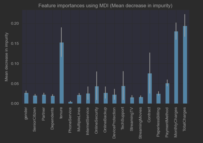
feature_names = X.columns.values.tolist()
importances = forest.feature_importances_
std = np.std([tree.feature_importances_ for tree in forest.estimators_], axis=0)
forest_importances_mdi = pd.Series(importances, index=feature_names)
RandomForest, GaussianNB, KNeighborsClassifier and LinearSVC
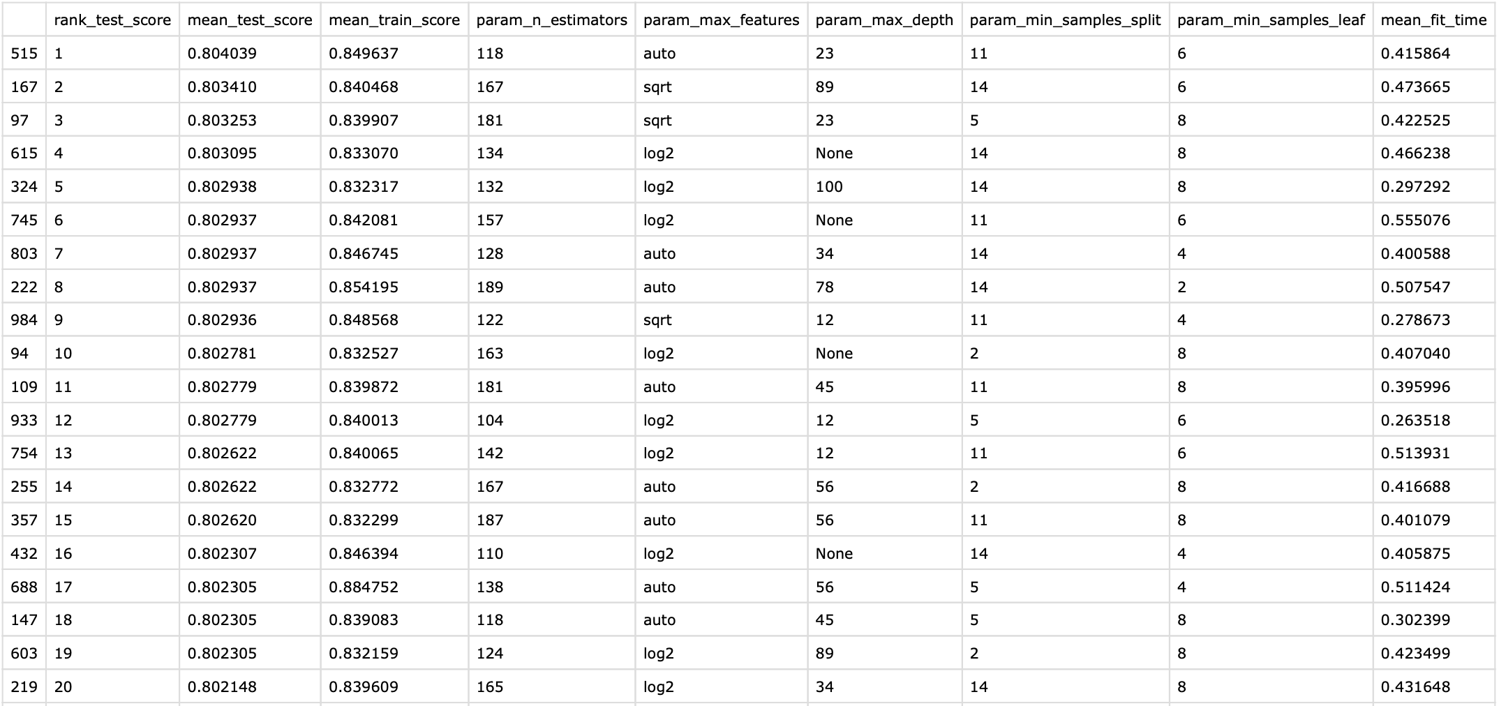
We searched with RandomSearch with N = 1000 iterations and found the following results below.
# Optimal Hyper-parameter Search using RandomSearch
parameters = {
    'n_estimators':[int(x) for x in np.linspace(start = 100, stop = 200, num = 50)],
    'max_depth': [int(x) for x in np.linspace(1, 100, 10)],
    'max_features': ['auto', 'sqrt','log2'],
    'min_samples_split': [2, 5, 8, 11, 14],
    'min_samples_leaf': [1, 2, 4, 6, 8],
    'max_samples': [float(2/3), 0.5, None],
}
parameters['max_depth'].extend([None])
parameters['n_estimators'].extend([10])

# Classifier
rf_clf = RandomForestClassifier(oob_score=True, n_jobs=-1)

# N-iterations
n_iterations = 1000

# 10-fold cross validation
k_fold = 10

# Columns to display
df_display_columns = ['rank_test_score', 'mean_test_score', 'mean_train_score', 'param_n_estimators', 'param_max_features', 'param_max_depth', 'param_min_samples_split', 'param_min_samples_leaf', 'mean_fit_time']

# Randomized Search
clf_rs = RandomizedSearchCV(estimator=rf_clf, param_distributions=parameters, cv=k_fold, return_train_score=True, scoring='accuracy', n_iter=n_iterations)
start = time.time()
search = clf_rs.fit(X_train, y_train)
stop = time.time()
df_rs = pd.DataFrame(clf_rs.cv_results_)

print('Best Parameters', search.best_params_, '\n')
print('RandomSearch Results, Ranked by Accuracy')
print(f'Total Fit Time: {round(stop - start, 2)}s')
print(f'N-Iterations: {n_iterations}')
display(HTML(df_rs[df_display_columns].sort_values('rank_test_score').to_html()))
{'n_estimators': 118, 'min_samples_split': 11, 'min_samples_leaf': 6, 'max_samples': 0.6666666666666666, 'max_features': 'auto', 'max_depth': 23}
We can see examples of underfitting, overfitting, and fitting well by altering parameters of the random forest algorithm.
-
Maximum Depth of Trees (max_depth):
- When trees are limited to only 1 level, it leads to underfitting due to a lack of complexity.
- When trees are not limited at all, they tend to overfit the training data, leading to lower scores on average.
- Optimum performance is achieved with a maximum depth of 2, striking a balance between complexity and overfitting.
-
Maximum number of Samples for bagging (max_samples):
- The number of instances added to a bootstrap sample to train a tree in the forest.
- The conventional recommendation is 2/3 of the input dataset, but in tests, 1/2 the length of the input and even 1/10 the length produced the same performance.
- Lower max_samples values result in quicker training times, which can be advantageous.
-
Maximum Features for each node (max_features):
- Controls the number of features chosen at random for each node split.
- Higher values reduce inter-tree correlation, making each tree's path to classification less likely to use the same feature selections.
- Testing showed that max_features=2 performed slightly better on average, but the differences between values for this hyperparameter were not significant.
## based on optimal hyper-parameters
best_params = {'n_estimators': 118, 'min_samples_split': 11, 'min_samples_leaf': 6, 'max_samples': float(2/3), 'max_features': 'auto', 'max_depth': 23}
default_params = { 'oob_score': True, 'n_jobs': -1 }
best_params.update(default_params)

rfc = RandomForestClassifier(**best_params)
rfc.fit(X_train,y_train)

# Get predictions
y_pred = rfc.predict(X_test)

# Confusion Matrix
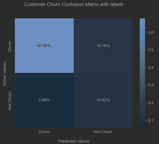
cf = skm.confusion_matrix(y_pred, y_test, normalize='all')
df_cm = pd.DataFrame(cf, index = ['Churn', 'Not Churn'],
                     columns = ['Churn', 'Not Churn'])

ax = sns.heatmap(df_cm, fmt='.2%', annot=True, cmap='Blues')
ax.set_xlabel('\nPredicted Values')
ax.set_ylabel('Actual Values ')
ax.set_title('Customer Churn Confusion Matrix with labels\n\n')

# Classification Report
print(skm.classification_report(y_pred, y_test))

plt.show()
              precision    recall  f1-score   support

           0       0.92      0.83      0.87       574
           1       0.48      0.68      0.56       131

    accuracy                           0.80       705
   macro avg       0.70      0.76      0.72       705
weighted avg       0.84      0.80      0.81       705
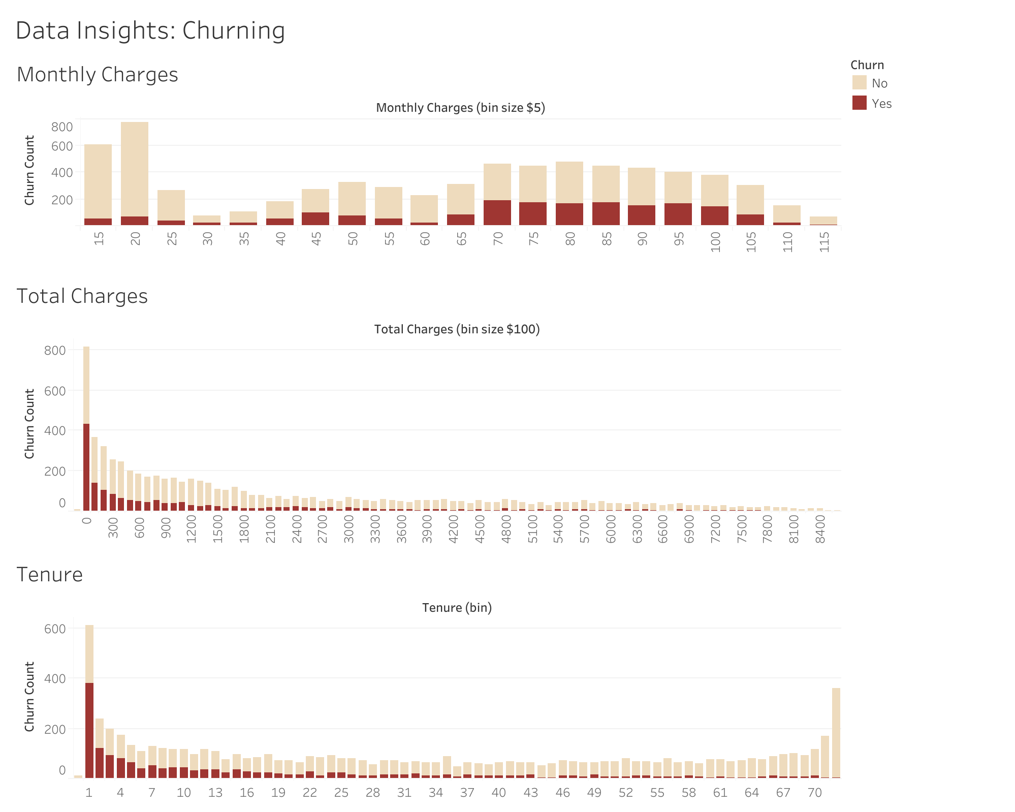
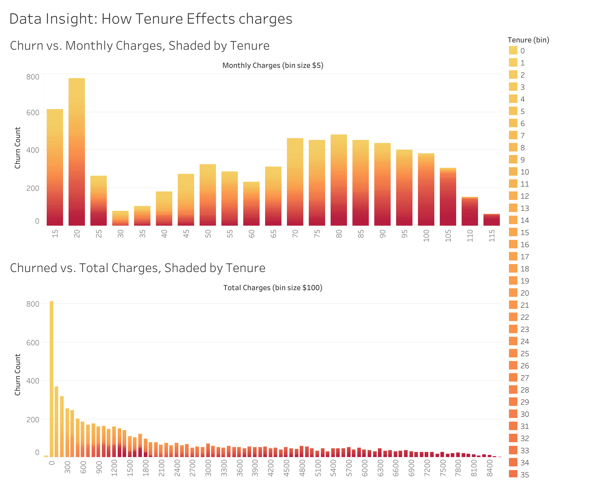
We can see clear trends in the data that tenure is inversley correlated with churning, which explains why low total charges shows a high churn rate.
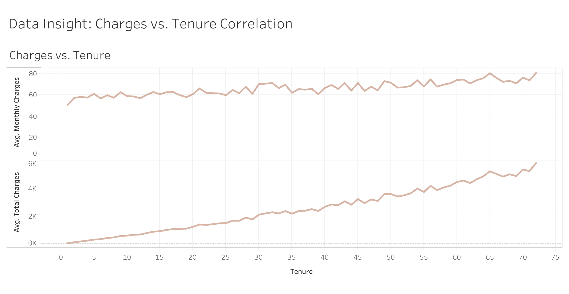
We can see that customers with long tenures tend to pay more monthly, and also have the most total charges over time.
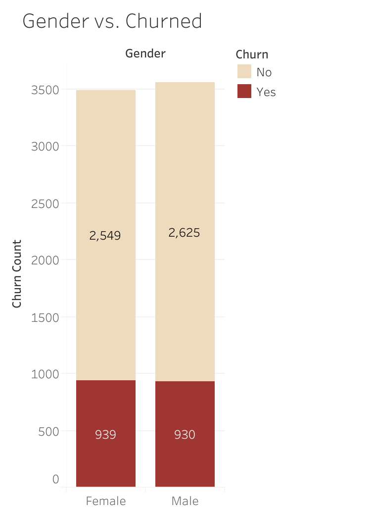
There are no significant differences in gender for churn rate.
