The complex system of vehicular runoff is studied with different models. Some macroscopic, which consider traffic as a continuum fluid, and some microscopic, which consider the relation of a driver with adjacent vehicles. Cell transmission model (CTM) is based on a class of macroscopic model called LWRs (Lighthill-Whitham-Richards model).
The variables of each macroscopic model are:
- flow
- density
- mean speed
which are connnected together by the hydrodynamic flow relation:
and also are subjected to a continuity equation:
The assunption of LWR models is that the flow is a funciton only of the density.
then:
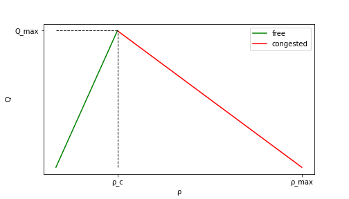
The flow-density relation is called fundamental diagram. CTM uses the simplest form of fundamental diagram, which has a triangular form:
The diagram has only two derivatives, which correspond to the only two possible speeds of propagation of the traffic wave. Above a critical density the wave will move upstream.
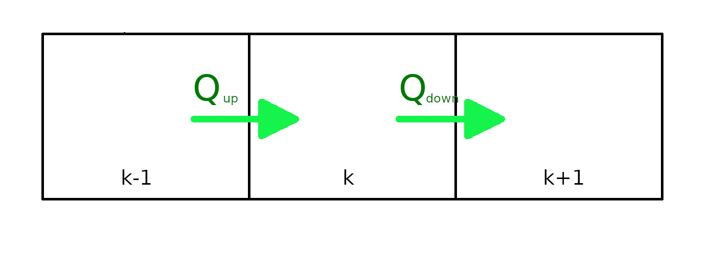
The numerical method consist in a discretization of space and time, then a recursive algorithm is applied:
-
compute supply and demand for each cell
-
determine flow at boundaries
-
update each cell density and total flow
To modify the flow in the road, for example if we want to simulate a speed limit or a traffic light or some bottlenekcks in general, we act on the capacity C of the cell. We will call the reduction in capacity bottleneck strength.
To start a simulation you have first to set the required parameters of the model which are divided in two section:
- model parameters (config.csv)
- bottlenecks parameters (bottlenecks.csv)
The necessary instructions are in the headers of the *.csv files. After compiling the configuration files you can run simulation.py from command line typing $python simulation.py -f <output_name> -p <configuration_file> -b <bottlenecks_file>.Flags corrspond respectively to --filename, --params and --bottlenecks.
e.g. $python simulation.py -f traffic_light -p configuration.csv -b bottlenecks.csv
A directory with name <output_name> is now created, it contains the configuration files and a png plot with with the density evolution of your road . If you will not pass a filename for your output the file will be named using the current date.
IMPORTANT: the road is always empty at the beginning, and is filled up in time proportional to the speed prameter.
-
plot.py only contains the function used to display the result
-
road.py contains the two classes used by the simulation:
Road creates a road object, which has all the model parameters, and that will be filled with cells
Cell creates a cell object, which has instead the physical variables we use to determine the density evolution
-
config.py has two functions for reading .csv files
images/ is just a folder for images used in README.md.
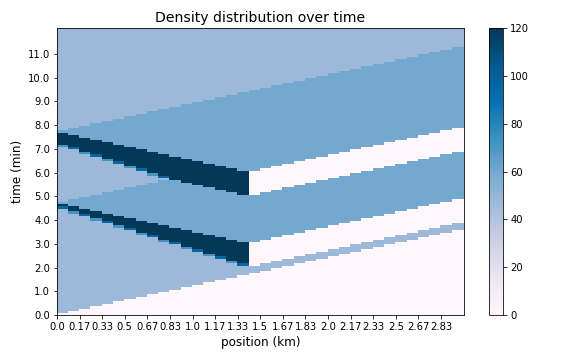
Here an example of simulation of a traffic light that turns red after 2 minute and after 5 minute.
| start | end | strenght | time_i | time_f |
|---|---|---|---|---|
| 1.5 km | 1.5 km | 1 | 2 min | 3 min |
| 1.5 km | 1.5 km | 1 | 5 min | 6 min |
| road_length | density_max | free_v | mean_time_gap | simulation_time | source | sink |
|---|---|---|---|---|---|---|
| 3 km | 120 veh/km | 50 km/h | 0.6 s | 0.2 h | 0.8 | 1 |
you can se how for the chosen source flow, the pause between the two red lights is not long enough for the traffic to flow out completely.


