Conduct financial event-study in just few lines of Python code.
What you need to provide is just a dataframe with events (ticker, event_date) - the rest leave to the Easy-Event-Study that will automatically:
- load and create returns time-series for the specified tickers
- load factors for the specified estimation model
- estimate abnormal returns for each event in the study
- provide the statistics table for each event with estimate AR and CAR
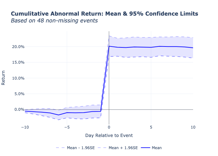
- plot mean cumulitative abnormal returns with specified confidence level.
Example of the event study output
The package could be easily installed with pip:
pip install easy_es
In order to use the library, one needs to provide a dataframe with events with just 2 columns:
- ticker - ticker name
- event_date - date to consider as the event for the specified ticker
from easy_es import EventStudy
from easy_es.utils import plot_mean_car, calculate_car_stats

# Event file should have 2 columns: ticker and event_date
events = pd.read_csv('events_df.csv')

event_study = EventStudy(
    estimation_days=255,
    gap_days=50,
    window_after=10,
    window_before=10,
    min_estimation_days=100,
    estimator_type='ff3',
    n_cores=1   # Number of CPU cores to use in processing. Usefull when there are many events
)
event_res_df = event_study.run_study(events_df)

# Get overall CAR stats with p-values
calculate_car_stats(event_res_df=event_res_df, critical_value=0.95)

# Plot mean effect with confidence levels
plot_mean_car(event_res_df=event_res_df, critical_value=0.95)
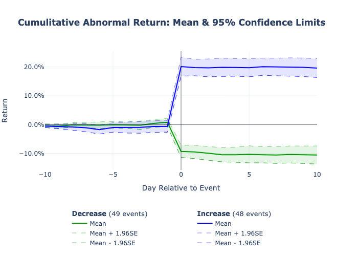
One could also plot the results of two event studies on the same graph, using:
from easy_es.utils import plot_joint_mean_car

event_res_increase = event_study.run_study(events_df_increase)
event_res_decrease = event_study.run_study(events_df_decrease)

plot_joint_mean_car(
    event_res_increase,
    event_res_decrease,
    name_one='Increase',
    name_two='Decrease'
)
Example of a joint mean CAR plot
All daily factors are downloaded for the official Fama-French data library.
Under the hood, Easy-Event-Study loads the returns data for the specified tickers and time-period using yfinance package.
Note: loading of returns might take a while depending on the size of the event-study. For example, for 400 tickers and 10 years - it takes around 10 mins.
Sometimes one needs to test several hypothesis with different combination of events. In order not to waste time on loading the returns data on every execution, one could do the following prior step before run_study:
## Load the returns. Dates should cover estimation and event windows
event_study.add_returns(
    list_of_tickers=events_df['ticker'].unique(),
    min_date='2010-01-01',  # Select min date to load returns from
    max_date='2023-01-01'   # Select max date to load returns until
)

## Get event study result for two different subsets of events.
event_res_one_df = event_study.run_study(events_df.head(100))
event_res_two_df = event_study.run_study(events_df.tail(100))
One could also dump the returns and load it back for the future executions:
## Load the returns. Dates should cover estimation and event windows
event_study.add_returns(
    list_of_tickers=events_df['ticker'].unique(),
    min_date='2010-01-01',  # Select min date to load returns from
    max_date='2023-01-01'   # Select max date to load returns until
)

event_study.returns_df.to_csv('returns_df.csv', index=False)

## Then load it back to the model in the future
event_study.add_returns(
    ret_df = pd.read_csv('returns_df.csv')
)
Methodology schema
For each event, define:- Estimation Period - when the parameters for the selected counterfactual model will be estimated.
- Gap Period - number of days to skip after estimation period
- Event window boundaries - number of days before and after an event to use in the calculations
Fit a selected model to estimate normal returns during the estimation period, and then construct abnormal returns (actual returns - normal return) during the event window.
Implemented models to estimate normal returns are:
-
CAPM -
$Ret_{i, t} = \alpha + \beta * (MktRet_{t} - RF_{t})$ , where-
$Ret_{i,t}$ - Return of company$i$ on day$t$ . -
$MktRet_{t}$ - Market return on day$t$ . -
$RF_{t}$ - Risk free rate on day$t$ .
-
-
Fama-French 3 factor model (aka FF3) -
$Ret_{i, t} = \alpha + \beta * (MktRet_{t} - RF_{t}) + \gamma * SMB_{t} + \theta * HML_{t}$ , where-
$Ret_{i,t}$ - Return of company$i$ on day$t$ -
$MktRet_{t}$ - Market return on day$t$ . -
$RF_{t}$ - Risk free rate on day$t$ . -
$SMB_{t}$ - Small minus Big factor on day$t$ . -
$HML_{t}$ - High minus Low factor on day$t$ .
-
-
Fama-French 5 factor model (aka FF5) -
$Ret_{i, t} = \alpha + \beta * (MktRet_{t} - RF_{t}) + \gamma * SMB_{t} + \theta * HML_{t} + \delta * CMA_{t} + \phi * RMW_{t}$ , where-
$Ret_{i,t}$ - Return of company$i$ on day$t$ -
$MktRet_{t}$ - Market return on day$t$ . -
$RF_{t}$ - Risk free rate on day$t$ . -
$SMB_{t}$ - Small minus Big factor on day$t$ . -
$HML_{t}$ - High minus Low factor on day$t$ . -
$CMA_{t}$ - Conservative Minus Aggressive factor on day$t$ . -
$RMW_{t}$ - Robust Minus Weak factor on day$t$ .
-
-
Market-Adjusted model (aka MAM) -
$Ret_{i, t} = MktRet_{t}$ , where-
$Ret_{i,t}$ - Return of company$i$ on day$t$ -
$MktRet_{t}$ - Market return on day$t$ .
-
To run the tests, run the following:
pytest tests/tests.py
The ground truth is obtained from an external EventStudy tool to verify that the difference between the results is close to zero.


