This project is a tutorial for RouteNet.
From the seminal paper Unveiling the potential of Graph Neural Networks for network modeling and optimization in SDN:
... RouteNet, a pioneering network model based on Graph Neural Networks (GNN), ... able to understand the complex relationship between topology, routing and input traffic to produce accurate estimates of the per-source/destination pair mean delay and jitter, ... to generalize over arbitrary topologies, routing schemes and variable traffic intensity.
This project is part of the joint MSc. in AI and Deep Learning dissertation project for Nathan Sowatskey and Ana Matute.
This project started as a GitHub fork of the demo paper Challenging the generalization capabilities of Graph Neural Networks for network modeling by J. Suárez-Varela, S. Carol-Bosch, K. Rusek, P. Almasan, M. Arias, P. Barlet-Ros and A. Cabellos-Aparicio.
The original authors of the demo paper provide a trained RouteNet model, in the form of Tensor Flow (TF) checkpoints, which may be found in the trained_models directory.
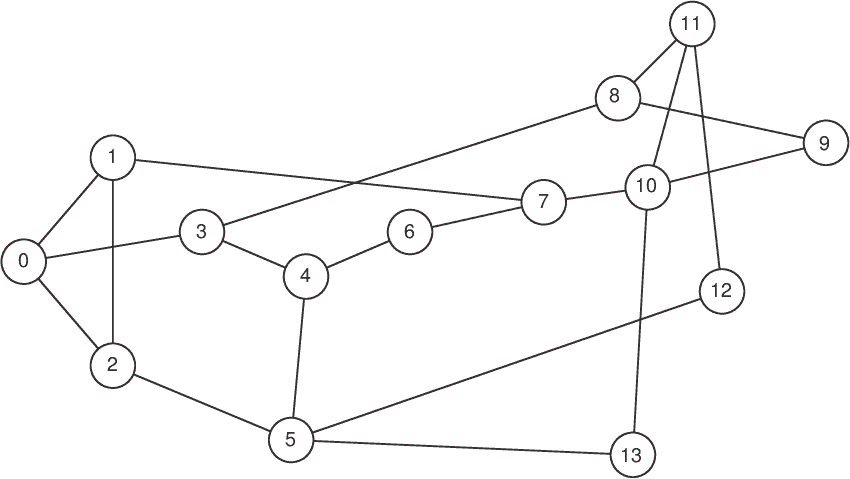
The pre-trained model is based on 480K training samples, including 240K samples from the 14-node NSF network topology
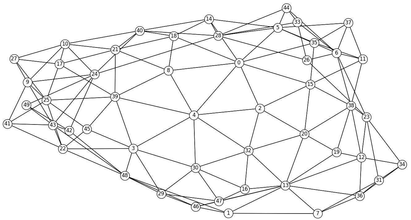
and 240K samples from the 50-node synthetically-generated topology.
The pre-trained model can be loaded to make per-source/destination delay predictions on any sample from the datasets, as demonstrated in the demo Jupyter notebook.
This project has a Travis Build.
The RouteNet Python package is in the src/routenet directory.
Unit and Smoke tests are in the tests directory.
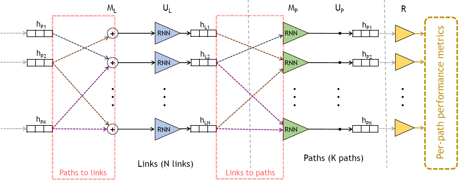
The following figure shows a schematic representation of the internal architecture of RouteNet. In this implementation, the input per-source/destination traffic is provided in the initial path states, while the link capacity is added as an input feature in the initial link states.
This model is implemented in routnet_model.py.
The original sample data sets were produced by a network simulator based on OMNet++ and are described in detail in OMNeT++ Data Files and Formats. How OMNeT++ was used to produce these data sets is outlined in section 4.1, "Simulation setup", of Unveiling the potential of Graph Neural Networks for network modeling and optimization in SDN, but there is no public means to replicate that part of the experiment.
To use this tutorial, you are strongly encouraged to set a Python virtual environment as explained below.
You can then obtain the original data sets, run the tests, then the training, and use the demo Python notebook to explore the prediction capabilities.
The scripts used in this tutorial rely on these two environment variables:
OMNET_DATA_DIR, which is the location of the network datasets data, within which the different dataset versions will be populated and obtained from.RN_PROJ_HOME, which is the full path name of thedemo-routenetdirectory cloned from GitHub, within which this file resides.
The virtual environment is created by the create_routenet_venv.sh and the set_routenet_venv.sh scripts. The create script will remove any existing virtual environment and create a new one, whilst the set script sets the environment thus created as the current environment. If the environment already exists, and does not need to be created afresh, then just the set script is required.
The Python packages required by the tutorial are defined in the requirements.txt file, which is passed to the Python pip tool as the environment is created.
The script uses the environment variable RN_PROJ_HOME, so ensure that is set before using these
scripts.
The get_omnet_data.sh script will retrieve and unpack the network datasets and update the test data for the smoke tests (see below).
The script uses two environment variables, OMNET_DATA_DIR and RN_PROJ_HOME, so ensure that they
are set before using this script.
The datasets obtained in the previous step already have the TFRecords version of the data, so you don't need to do this. If you want to see how that conversion works, for the sake of curiosity say, then the process_omnet_data_v0.py script will do that.
There are two kinds of tests provided:
- Unit tests, in the tests/unit, which individually test the TFRecord conversion, training and model prediction, and which execute in he order of a couple of minutes or less.
- Smoke tests, which run through the lifecycle of TFRecord conversion, train and predict, for some hundreds of iterations, and which can take several hours to to execute.
To get quicker results from the smoke tests, you can comment out the tests for the geant2bw and
synth50bw datasets, so that the tests just run with the nsfnetbw dataset. This will execute in the
order of tens of minutes, but is obviously slightly less thorough.
It is highly recommended to run the tests, which use subsets of the datasets, before you start to use the model for training with the full datasets. If your environment is not set up properly, or the code is broken somehow, then the running the tests will quickly reveal that.
The train_multiple_v0.py script runs the training. The script can be
adjusted to train and evaluate with different data sets, and for different numbers of iterations.
The checkpoints for any given combination of datasets and training iterations will be saved in a
directory named with that combination. For example, the directory
model_checkpoints-train_nsfnetbw_geant2bw-eval_synth50bw-50000_v0 contains
checkpoints, and evaluation logs, for a training run of 50,000 iterations with the train subset of the
nsfnetbw and geant2bw data sets, evaluated against the evaluation subset of the synth50bw
dataset.
TensorBoard is TensorFlow's visualization toolkit. You can use TensorBoard during training, and after, to view the evaluation data for the model over training iterations.
The evaluation log data is in the eval sub-directory of the checkpoints directory. For example,
if you are training, using 50,000 iterations, with the nsfnetbw and geant2bw datasets, and
evaluating with the synth50bw data set, then the evaluation logs will be in the
model_checkpoints-train_nsfnetbw_geant2bw-eval_synth50bw-50000_v0 directory. To use TensorBoard,
then, you can use the commands below. Note that the eval directory will only exist ten minutes after
the training has started, as a consequence of the setting throttle_secs=10 * 60 in the training code.
cd $RN_PROJ_HOME/model_checkpoints-train_nsfnetbw_geant2bw-eval_synth50bw-50000_v0/eval
tensorboard --logdir .
Then you can open the TensorBoard web application in a browser at 'http://localhost:6006/' and see the logs via a web application.
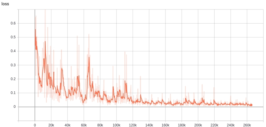
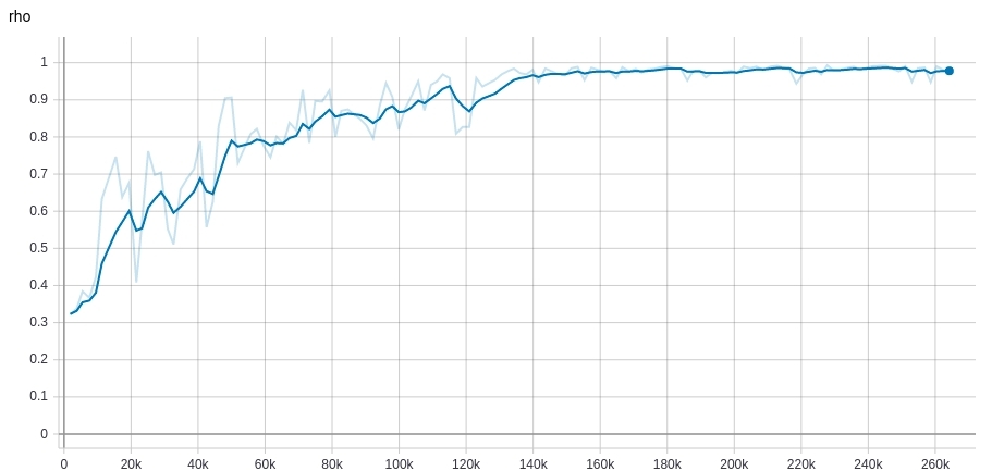
As an example, the figures below show the evolution of the loss (Mean Absolute Error) and the accuracy (Pearson correlation coefficient) of the RouteNet model that is provided in the 'trained_models' directory.
This model was trained with samples of the 14-node NSFNET and the 50-node topologies, and was evaluated over samples of the Geant2 topology.
The prediction demo notebook uses different checkpoints to illustrate the prediction capabilities.
