This branch is no longer developed. The actively developed branch is https://github.com/vemiBGH/PULSEE.
PULSEE is an open-source software for the simulation of typical nuclear quadrupole/magnetic resonance experiments on a solid-state sample, describing the dynamics of nuclear spins in condensed matter under the effect of external magnetic fields and reproducing the traditional results observed in laboratory.
Each atomic nucleus in a single crystal is endowed with an intrinsic angular momentum, named spin, and a corresponding intrinsic magnetic moment. The interaction between this latter and any applied magnetic field provides a means for the manipulation of nuclear spins and the study of nuclear interactions in a material.
The basic assumption of the simulations implemented with this program is that the nuclei belonging to the sample under study are identical and independent, so that the set of all their spins can be treated as an ideal statistical ensemble: this allows to describe the state of the whole many-spin system with a mixed density matrix of dimensions 2s+1, where s is the quantum numer of a single spin.
Let us consider such a system under the effect of a static magnetic field. In these circumstances, the degeneracy of spin states is broken and they arrange into equally spaced energy levels, with an energy separation determined by the strength of the field and the gyromagnetic ratio of the nuclear spin.
In order to induce transitions between these states, a pulsed electromagnetic wave must have a frequency tuned with the resonance frequency of the system. This is the concept at the basis of the nuclear magnetic resonance (NMR) technique.
In nuclear quadrupole resonance (NQR), what breaks the degeneracy of spin states is the interaction between the electric quadrupole moment of the nucleus and the electric field gradient (EFG) generated by surrounding electrons. The applied electromagnetic pulses are able to induce an appreciable change in the state of the system only if their frequency is in resonance with one of the frequencies of transition.
In general, experimental systems are characterized by an intermediate configuration where both a magnetic field and an EFG are present and the corresponding interactions must be taken into account simultaneously in order to determine the energy spectrum.
In order to extract information about the interactions of nuclear spins and the properties of the crystal structure, NMR and NQR represent successful techniques of investigation. Indeed, after the application of a given pulse sequence, the system's magnetization typically developes a non-zero component along the direction of the coil employed for the generation of the pulse. This component changes with time in a way that depends on the energy spectrum of the nuclei, while it progressively goes to zero due to the unavoidable dephasing of different spins, which takes place with a characteristic time T2 (coherence time).
The time dependence of the magnetization is measured through the acquisition of the current it induces in the coil. Then, performing the Fourier analysis of this signal, one is able to extract a lot of information about the system, according to the position of the peaks of the spectrum, their shape and their sign.
In order to save processing power and lighten calculations, a suitable choice of units of measure has been taken.
Remark: In the whole software, energies and frequencies are considered quantities with the same physical dimensions. The identification between them is a consequence of setting the Planck constant h equal to 1.
The standard units employed in the software are listed below.
| physical quantity | unit |
|---|---|
| gyromagnetic ratio | MHz/T |
| magnetic field | T |
| energy/frequency | MHz |
| temperature | K |
| time | us |
Angles do not have a standard unit: they are measured in radians when they are passed directly to the software's functions, while they are measured in degrees when they are inserted in the GUI.
PULSEE has been written in Python 3.7.
The operative systems where it has been tested and executed are
- Ubuntu
- Windows 10 (through the Spyder interface provided by the distribution Anaconda)
The software makes wide use of many of the standard Python modules (namely numpy, scipy, pandas, matplotlib) for its general purposes.
Tests have been carried out using the pytest framework and the hypothesis module.
pytest -> https://docs.pytest.org/en/stable/
hypothesis -> https://hypothesis.readthedocs.io/en/latest/
The GUI has been implemented with the tools provided by the Python library kivy.
kivy -> https://kivy.org/#home
In order to run the GUI, it is required the additional installation of the module kivy.garden and garden.matplotlib.backend_kivy.
Remark: The package garden.matplotlib.backend_kivy is only compatible with matplotlib 3.1 or older.
kivy.garden -> https://kivy.org/doc/stable/api-kivy.garden.html
garden.matplotlib.backend_kivy -> https://github.com/kivy-garden/garden.matplotlib/blob/master/backend_kivy.py
PULSEE is made up by 6 modules. Each of them is described in full detail in the wiki page of the repository of GitHub which hosts the project:
https://github.com/DavideCandoli/NQR-NMRSimulationSoftware/wiki
Below, the content and usage of these modules is reported briefly:
-
OperatorsThis module, together with
Many_Body, is to be considered a sort of toolkit for the simulations of generic quantum systems. It contains the definitions of classes and functions representing the basic mathematical objects employed in the treatment of a quantum system.Operatorsfocuses on the properties of a single system, while the functions inMany_Bodyallow to build up systems made up of several particles.The classes and subclasses defined in
Operatorsbelong to the following inheritance treeOperatorDensity_Matrix(Operator)Observable(Operator)
Class
Operatordefines the properties of a generic linear application acting in the Hilbert space of a finite-dimensional quantum system. Its main attribute ismatrix, a square array of complex numbers which gives the matrix representation of the operator in a certain basis. The methods of this class implement the basic algebraic operations and other common actions involving operators, such as the change of basis.Class
Density_Matrixcharacterizes the operators which represent the state (pure or mixed) of the quantum system. It is defined by three fundamental properties:- hermitianity
- unit trace
- positivity
Class
Observablecharacterizes the hermitian operators which represent the physical properties of the system.Other functions defined in this module perform:
- the calculation of the first few terms of the Magnus expansion of a time-dependent Hamiltonian, which enter the approximate formula for the evolution operator;
- the calculation of the canonical density matrix representing the thermal equilibrium state of a system at the specified temperature.
-
Many_BodyThis module defines two functions which allow to pass from a single particle Hilbert space to a many particle space and viceversa.
-
tensor_productTakes two operators of arbitrary dimensions and returns their tensor product.
-
partial_traceTakes an operator acting on the Hilbert space of a many-particle system and extracts its partial trace over the specified subspace.
-
-
Nuclear_SpinIn this module, the objects defined in
Operatorsare employed to build up the class which represents the spin of an atomic nucleus or a system of nuclei.Class
Nuclear_Spinis characterized by a quantum number, a gyromagnetic ratio and a set of methods which return the spherical and cartesian components of the spin vector operator.The subclass
Many_Spinscontains theNuclear_Spinobjects representing the individual spins in a system of many nuclei, as well as a method for the calculation of the operators of the total spin. -
HamiltoniansThis file is dedicated to the definitions of the functions which compute the terms of the Hamiltonian of a nuclear spin system in a NMR/NQR experiment.
-
h_zeemanBuilds up the Hamiltonian of the interaction between the spin and an external static magnetic field, after its magnitude and direction have been given.
-
h_quadrupoleBuilds up the Hamiltonian of the interaction between the nuclear electric quadrupole momentum and the EFG, after the coupling constant of the interaction, the asymmetry of the EFG and the direction of its principal axes have been given.
In its scope,
h_quadrupolecalls the three functionsv0_EFG,v1_EFG,v2_EFGin order to compute the spherical components of the EFG tensor, which enter the expression of the quadrupole Hamiltonian. -
h_single_mode_pulseReturns the Hamiltonian of interaction of a nuclear spin with a linearly polarized electromagnetic wave, once the properties of the wave and the time of evaluation have been passed.
This function is iterativily called by
h_multiple_mode_pulse, which returns the Hamiltonian of interaction between a nuclear spin system and a superposition of pulses.In turn,
h_multiple_mode_pulseis called insideh_changed_picture, which, in the given instant of time, evaluates the full Hamiltonian of the system (comprised of the Zeeman, quadrupole and time-dependent contributions) and returns the same Hamiltonian expressed in a different dynamical picture. This passage is required by the implementation of the evolution of the system, which is described later.
-
-
SimulationThis module provides the definition of the functions which implement the various tasks of the simulation. A user whose aim is to perform simulations of the kind of the examples which follow just needs to learn how to use the functions in this module. More sophisticated simulations are feasible, but they require a deeper knowledge of the features of the program, as the user should deal directly with the definitions in the other modules.
The order in which the definitions in
Simulationappear suggests the ideal progression of the various steps of the simulation.-
nuclear_system_setupBuilds up the system under study, creating the objects associated with the nuclear spin system, the unperturbed Hamiltonian (Zeeman + quadrupole contributions) and the initial state.
-
power_absorption_spectrumComputes the power absorbed by the system from a pulse as a function of the frequency of the pulse, according to the theoretical formula derived from Fermi golden rule.
-
evolveEvolves the state of the system under the action of a given electromagnetic pulse, or just the stationary Hamiltonian. Evolution is carried out approximating the evolution operator with the first terms of the Magnus expansion and the user can specify in which dynamical picture to evolve the system.
-
FID_signalSimulates the free induction decay signal generated by the transversal magnetization of the system after the application of a pulse.
-
fourier_transform_signalPerforms the Fourier analysis of a signal (in this context, the FID).
-
fourier_phase_shiftComputes the phase shift to be applied to the FID in order to correct the shape of the Fourier spectrum of the system and recover the typical absorptive/dispersive lorentzian shapes at a given peak.
Besides these functions, which execute the main passages of the simulation, this module contains the functions for the plot and visualization of the results.
-
-
PULSEE_GUIGraphical user interface of the program. The execution of the following command from the terminal
$ python PULSEE_GUI.pylaunches the application. This has been developed using the tools provided by the library Kivy.
In the application, most of the features of the software are available, but not all of them (for instance, power absorption spectra are not included). An in-depth description of the GUI can be found in the related page of the wiki:
Any simulation can be implemented using only the functions defined in the module Simulation. Therefore, the imports required by a generic simulation code are the following:
from Simulation import nuclear_system_setup, \
                       evolve, \
                       power_absorption_spectrum, \
                       plot_power_absorption_spectrum, \
                       plot_real_part_density_matrix, \
                       FID_signal, \
                       plot_real_part_FID_signal, \
                       fourier_transform_signal, \
                       fourier_phase_shift, \
                       plot_fourier_transform
The simplest experiment one can simulate is the case of pure NMR, where a static magnetic field (conventionally directed along z) is applied to a nucleus where the quadrupolar interaction is negligible.
Take for instance a spin 1 nucleus: the set up of the system is carried out passing to nuclear_system_setup the following parameters:
spin_par = {'quantum number' : 1.,
            'gamma/2pi' : 1.}

zeem_par = {'field magnitude' : 1.,
            'theta_z' : 0.,
            'phi_z' : 0.}

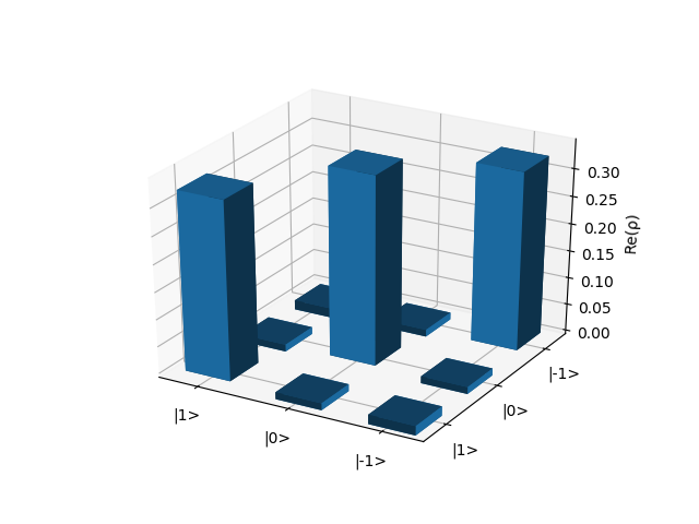
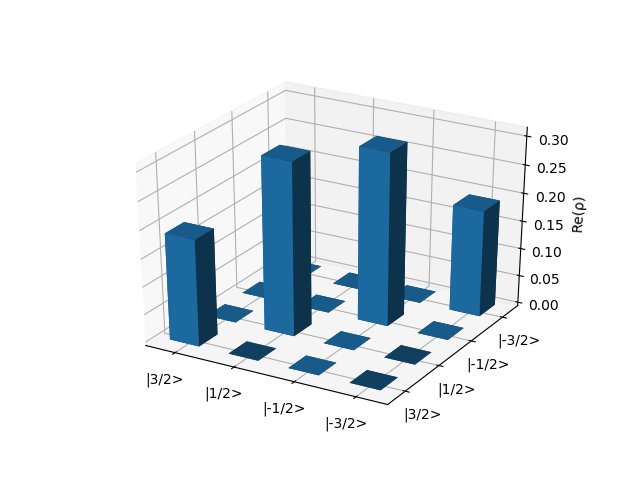
spin, h_unperturbed, dm_0 = nuclear_system_setup(spin_par=spin_par, quad_par=None, zeem_par=zeem_par, initial_state='canonical', temperature=1e-4)

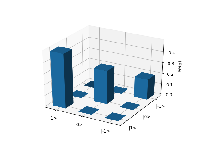
plot_real_part_density_matrix(dm_0)
where the system has been initially set at thermal equilibrium at a temperature of 10-4 K.
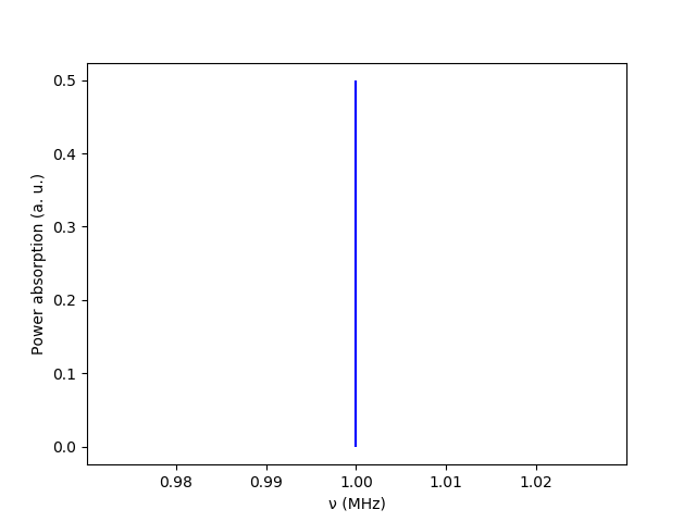
Then, the power absorption spectrum can be simulated running the functions
f, p = power_absorption_spectrum(spin, h_unperturbed, normalized=True)

plot_power_absorption_spectrum(f, p)
In order to apply a 90° pulse to the system, which rotates the magnetization from the z-axis to the x-y plane, we shall design a pulse in resonance with the system such that the product
gyromagnetic ratio x pulse field magnitude x pulse time
is equal to pi/2. Setting a pulse made up of the single linearly polarized mode
mode = pd.DataFrame([(1., 0.1, 0., math.pi/2, 0.)],
                     columns=['frequency', 'amplitude', 'phase', 'theta_p', 'phi_p'])
the pulse time should be equal to 5 us in order to produce a 90° rotation. Indeed, the effective amplitude of the wave is 0.05 T: the linearly polarized mode splits into two rotating waves, only one of which is in resonance with the system.
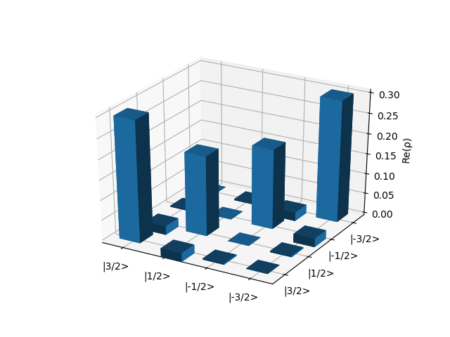
Then, the state of the system is evolved and plotted with the following calls:
dm_evolved = evolve(spin, h_unperturbed, dm_0, \
                    mode=mode, pulse_time=5, \
                    picture = 'IP')

plot_real_part_density_matrix(dm_evolved)
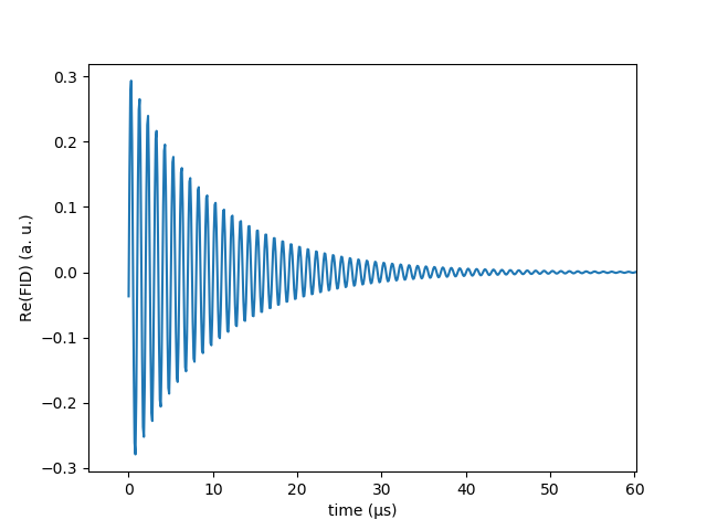
The evolved density matrix can be employed to generate the FID signal of the system as follows:
t, fid = FID_signal(spin, h_unperturbed, dm_evolved, acquisition_time=100, T2=10)

plot_real_part_FID_signal(t, fid)
Remark: In order to acquire a true reproduction of the continuous FID signal, one needs to compare the largest frequency in its Fourier spectrum with the frequency of sampling of the signal. Indeed, Nyquist theorem states that the latter must be at least twice the former to ensure a correct sampling. See the documentation for FID_signal to learn how to set the number of sampling points.
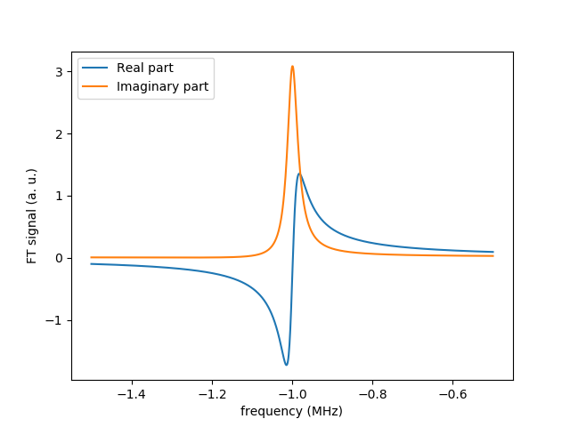
The Fourier analysis of the FID signal produces the NMR spectrum:
f, ft = fourier_transform_signal(t, fid, -1.5, -0.5)

plot_fourier_transform(f, ft)
When the quadrupolar interaction is non-negligible, but still very small compared to the interaction with the magnetic field, one is in the so-called perturbed Zeeman regime.
An experiment with these conditions can be easily simulated following the same steps described in the pure Zeeman case with the only difference being a non-zero quadrupolar coupling constant:
quad_par = {'coupling constant' : 0.2,
            'asymmetry parameter' : 0.,
            'alpha_q' : 0.,
            'beta_q' : 0.,
            'gamma_q' : 0.}

spin, h_unperturbed, dm_0 = nuclear_system_setup(spin_par=spin_par, quad_par=quad_par, zeem_par=zeem_par, initial_state='canonical', temperature=1e-4)
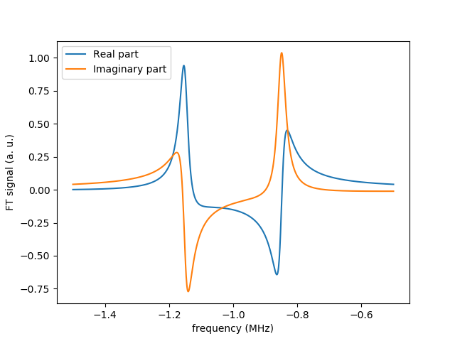
The presence of this perturbation leads eventually to a spectrum with two resonance peaks.
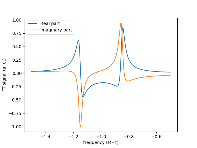
As one can see, the real and imaginary parts of the spectrum at each peak don't fit the conventional absorptive/dispersive lorentzian shapes, which would be a nice feature to be visualized. By means of the function fourier_phase_shift, one can obtain the phase for the correction of the shape of the spectrum at a specified peak (the simultaneous correction at both peaks is impossible):
phi = fourier_phase_shift(f, ft, peak_frequency=-0.82, int_domain_width=0.2)

plot_fourier_transform(f, np.exp(1j*phi)*ft)
Another important type of experiments is that of pure NQR, where the only term of the unperturbed Hamiltonian is the quadrupolar interaction. The pure NQR of spin 3/2 nuclei can be simulated changing the parameters in the previous two examples as
spin_par = {'quantum number' : 3/2,
            'gamma/2pi' : 1.}

quad_par = {'coupling constant' : 2.,
            'asymmetry parameter' : 0.,
            'alpha_q' : 0.,
            'beta_q' : 0.,
            'gamma_q' : 0.}

spin, h_unperturbed, dm_0 = nuclear_system_setup(spin_par=spin_par, quad_par=quad_par, zeem_par=None, initial_state='canonical', temperature=1e-4)
where we have set the coupling constant of the quadrupole interaction to 2 MHz.
In such a configuration, the pulse set up in the previous example turns to be in resonance with the new system as well, so that it can be left unaltered.
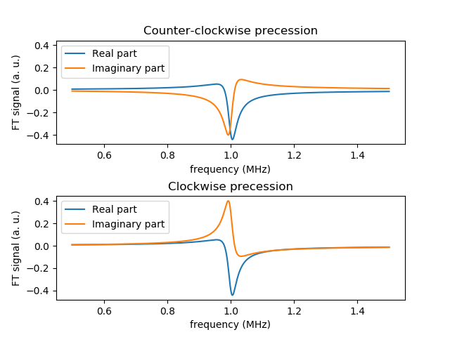
In this case, the frequencies of transition of the system have same modulus but opposite sign, namely 1 and -1 MHz. This means that both the rotating waves that make up the linearly polarized pulse are able to induce transitions. In order to visualize properly both the positive and negative resonance lines in the spectrum, the functions for the analysis of the FID must be run with the following parameters:
f, ft, ft_n = fourier_transform_signal(t, fid, 0.5, 1.5, opposite_frequency=True)

plot_fourier_transform(f, ft, ft_n)
The program presented above was made possible thanks to professors Samuele Sanna (Università di Bologna) and Vesna Mitrovic (Brown University), who have been a great help in the interpretation of the physics simulated by the software.
Further contributions to the developement of the program have been the advices given by Stephen Carr (Brown University) and professor Enrico Giampieri (Università di Bologna).
