Devinterview-io/k-means-clustering-interview-questions

🟣 K Means Clustering interview questions and answers to help you prepare for your next machine learning and data science interview in 2025.

50 Common K-Means Clustering Interview Questions in 2025

You can also find all 50 answers here 👉 Devinterview.io - K-Means Clustering

1. What is K-Means Clustering, and why is it used?

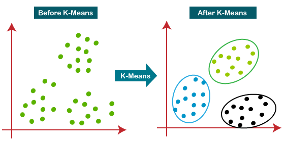
K-Means Clustering is one of the most common unsupervised clustering algorithms, frequently used in data science, machine learning, and business intelligence for tasks such as customer segmentation and pattern recognition.

Core Principle

K-Means partitions data into $k$ distinct clusters based on their attributes. The algorithm works iteratively to assign each data point to one of $k$ clusters, aiming to minimize within-cluster variances.

Key Advantages

• Scalability: Suitable for large datasets.

• Generalization: Effective across different types of data.

• Performance: Can be relatively fast, depending on data and $k$ value choice. This makes it a go-to model, especially for initial exploratory analysis.

Limitations

• Dependence on Initial Seed: Results can vary based on the starting point, potentially leading to suboptimal solutions. Using multiple random starts or advanced methodologies like K-Means++ can mitigate this issue.

• Assumes Spherical Clusters: Works best for clusters that are somewhat spherical in nature. Clusters with different shapes or densities might not be accurately captured.

• Manual $k$ Selection: Determining the optimal number of clusters can be subjective and often requires domain expertise or auxiliary approaches like the elbow method.

• Sensitive to Outliers: Unusually large or small data points can distort cluster boundaries.

Measures of Variability

Within-cluster sum of squares (WCSS) evaluates how compact clusters are:

$$ \text{WCSS} = \sum_{i=1}^{k} \sum_{x \in C_i} ||x - \mu_i||^2 $$

Where:

• $k$ is the number of clusters.
• $C_i$ represents the $i$th cluster.
• $\mu_i$ is the mean of the $i$th cluster.

Evaluation Metrics

Silhouette Coefficient

The silhouette coefficient measures how well-separated clusters are. A higher value indicates better-defined clusters.

$$ s(i) = \frac {b(i) - a(i)} { \max{a(i), b(i)}} $$

Where:

• $a(i)$: Mean intra-cluster distance for $i$ relative to its own cluster.
• $b(i)$: Mean nearest-cluster distance for $i$ relative to other clusters.

The silhouette score is then the mean of each data point's silhouette coefficient.

2. Can you explain the difference between supervised and unsupervised learning with examples of where K-Means Clustering fits in?

K-Means Clustering falls under unsupervised learning, in contrast to supervised learning methods like Decision Trees and Random Forest.

Unsupervised Learning: Discovering Patterns

In unsupervised learning, the algorithm doesn't rely on labeled data and operates by identifying commonalities or patterns in the dataset. This method is more about exploration and understanding.

K-Means Clustering: Grouping Data

K-Means is a partition-based method, clustering data by minimizing the Euclidean distance between each point and the centroid of its associated cluster.

Example: A real-world application is in customer segmentation, where similar customers are grouped together based on their shopping behavior.

Supervised Learning: Assigning Labels

Supervised learning is all about teaching a model how to map input to output based on example data. The model then uses that knowledge to predict the correct output when presented with new input.

Decision Trees: Classification and Regression

A Decision Tree sequentially segments the data in a tree-like structure. At each node, the tree makes a decision that best separates the data based on certain features.

Example: Decision Trees can be used in medicine to diagnose patients based on symptoms.

Random Forest: Ensemble Learning

Random Forest is an ensemble of Decision Trees. It constructs several trees through bootstrapping, each considering a subset of features, and combines their predictions through voting (for classification) or averaging (for regression).

Example: A practical application is in predicting customer churn for businesses.

3. What are centroids in the context of K-Means?

In k-Means clustering, centroids represent data points that act as the center of clusters. Each cluster is defined by its corresponding centroid, and the goal of the algorithm is to minimize intra-cluster distances by optimizing these centroids.

Role of Centroids

• Cluster Assignment: Each data point is associated with the closest centroid, effectively linking it to a specific cluster.
• Initial Centroid Selection: Starting with an initial guess, the algorithm iteratively updates these points. Convergence occurs when the centroids no longer shift substantially.
• Model Representation: The optimized centroids, alongside the assigned data points, define the k-Means model. This model can make inferences about future, unseen data by assigning them to the nearest centroids.

Centroid Calculation

Mathematically, the centroid of a cluster $C_k$ having $n_k$ data points in a $d$-dimensional space is given by the mean of the data points in that cluster:

The algorithm aims to find centroids that minimize the within-cluster sum of squares (WCSS), which is also known as inertia. This is measured by:

The smaller this value, the better the clustering.

4. Describe the algorithmic steps of the K-Means clustering method.

K-Means is a straightforward and widely-used clustering algorithm. It partitions $n$ data points into $k$ groups ($k$ is predetermined) through an iterative process.

Visual Representation

Algorithm Steps

1. Initialize

   • Randomly pick $k$ initial centroids ($k$ distinct data points).
   • Assign each data point to the nearest centroid, forming $k$ clusters.

2. Update Centroids

   Recalculate the centroids of newly formed clusters.

3. Reassign Points

   Reassign each data point to the nearest centroid.

4. Iterate

   Steps 2 and 3 are repeated till:

   • No change in centroids.
   • Given the tolerance, the algorithm stops.

Code Example: K-Means Steps

Here is the Python code:

# Initialize
from sklearn.datasets import make_blobs
import numpy as np

X, _ = make_blobs(n_samples=300, centers=4, cluster_std=0.60, random_state=0)

k=4
centroids = X[np.random.choice(X.shape[0], k, replace=False)]
print('Initial Centroids:', centroids)

# Update centroids
def update_centroids(X, centroids):
    clusters = [[] for _ in range(k)]
    for point in X:
        distances = [np.linalg.norm(point - centroid) for centroid in centroids]
        cluster_idx = np.argmin(distances)
        clusters[cluster_idx].append(point)
    
    for i in range(k):
        centroids[i] = np.mean(clusters[i], axis=0)

    return centroids, clusters

# Reassign Points - visual representation
import matplotlib.pyplot as plt

def plot_clusters(X, centroids, clusters):
    colors = ['b', 'g', 'r', 'c', 'm', 'y', 'k']
    for i in range(k):
        plt.scatter(centroids[i][0], centroids[i][1], s=300, c=colors[i], marker='o', label=f'Centroid {i+1}')
        cluster_points = np.array(clusters[i])
        plt.scatter(cluster_points[:,0], cluster_points[:,1], c=colors[i], label=f'Cluster {i+1}')

    plt.scatter(X[:,0], X[:,1], c='gray', alpha=0.2)
    plt.legend()
    plt.show()

# First Iteration
centroids, clusters = update_centroids(X, centroids)
plot_clusters(X, centroids, clusters)

5. What is the role of distance metrics in K-Means, and which distances can be used?

Distance metrics play a pivotal role in K-Means clustering. They are fundamental for determining cluster assignments and optimizing cluster centers iteratively.

Distances in K-Means

1. Euclidean Distance

The most commonly used distance metric in K-Means, based on the formula:

$$ \sqrt{\sum_{i=1}^{n}{(x_i - y_i)^2}} $$

where $x_i$ and $y_i$ represent the data points' orthogonal coordinates.

2. Manhattan (Taxicab) Distance

Defined as the sum of the absolute differences between the coordinates:

$$ \sum_{i=1}^{n}{\lvert x_i - y_i \rvert} $$

This metric evaluates distance in grid-based systems, where movement occurs along coordinate axes.

3. Chebyshev Distance

Also known as chessboard distance, it represents the maximum absolute difference between corresponding coordinates along the axes, given by:

$$ \max_{i}(\lvert x_i - y_i \rvert) $$

4. Minkowski Distance

Generalizing both Euclidean and Manhattan distances, Minkowski distance is parameterized by a value $p$ and described as:

$$ \left( \sum_{i=1}^{n}{\lvert x_i - y_i \rvert^p} \right)^{1/p} $$

When $p = 2$, it simplifies to the Euclidean distance, and for $p = 1$, it reduces to the Manhattan distance.

6. How do you decide on the number of clusters (k) in a K-Means algorithm?

Choosing the right number of clusters $k$ is vital for the effectiveness of K-Means and impacts the interpretability of the clusters. Here are some popular methods for guidance:

Visual Inspection

Inspect k-means results across a range of cluster counts to identify a suitable $k$ via visual clues. Plot metrics such as inertia and silhouette score across different values of $k$ to aid in this process.

The Elbow Method

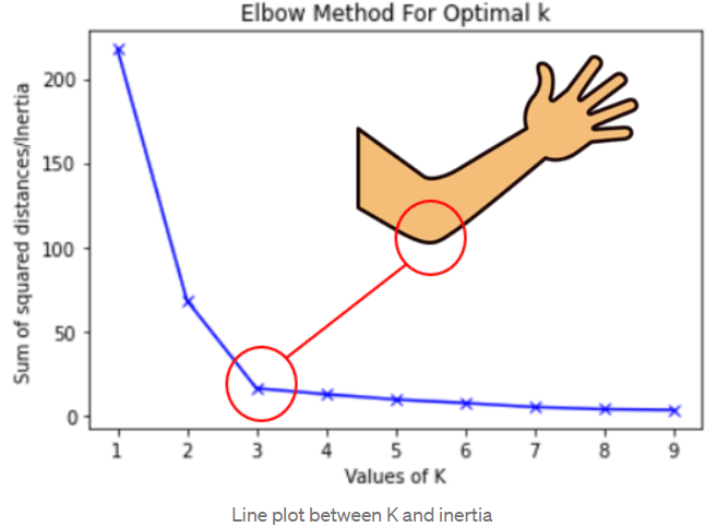
In the Elbow method, one looks for the $k$ value where the rate of inertia change sharply decreases, resembling an "elbow" shape. While this method can provide a reasonable estimate, the "elbow" is not always distinctly visible.

The Silhouette Method

The Silhouette score gauges how well-separated the resulting clusters are. A higher silhouette score indicates better-defined clusters.

One can compute the silhouette score for various $k$ values and choose the $k$ that gives the highest score.

The Gap Statistic Method

The Gap Statistic evaluates the consistency of clustering in datasets, looking for the first $k$ where additional clusters do not add significantly more information. It does so by comparing the original inertia with a distribution of inertias generated from random data.

The Dendrogram Method

This approach, often employed in hierarchical clustering but also adaptable for K-Means via the Agglomerative Nesting algorithm, utilizes a tree diagram or dendrogram to show the arrangement of clusters.

One can then look for the level in the dendrogram that has the longest vertical lines not intersected by any cluster merges. This represents an optimal number of clusters.

Cross-Validation

Techniques such as k-fold cross-validation can provide estimates for the best $k$ through measures like mean square error or silhouette score.

Model-Based Methods

Methods like Gaussian Mixture Models use a data-driven approach, utilizing probabilistic assignments and the Bayesian Information Criterion (BIC) or Akaike Information Criterion (AIC) to assess model fit. Other methods focus on subspace clustering or use dimensionality reduction techniques before clustering to estimate the right number of clusters.

7. What are some methods for initializing the centroids in K-Means Clustering?

K-Means Clustering efficiency rests on strong initial centroid selection. Incorrect initial seeding might lead to suboptimal cluster separation or slow convergence. Here are the common centroid initialization methods.

K-Means++

K-Means++ enhances the random approach by probabilistically selecting the initial centroids. This initiative lessens the likelihood of starting with close or outlier centroids.

1. Algorithm:

   • Choose the first centroid randomly from the dataset.
   • For every next centroid, pick a sample with a likelihood of being selected proportional to its squared distance from the closest centroid.
   • Keep repeating this procedure until all centroids are chosen.

2. Advantages:

   • Suited for large datasets.
   • Still relatively efficient even when $k$ (the number of clusters) is not small.

3. Code Example: Here is the Python code:

   from sklearn.cluster import KMeans
   kmeans = KMeans(n_clusters=4, init='k-means++')

K-Means

K-Means is the classic approach where the initial centroids are randomly picked from the dataset.

1. Random Sampling:

   • Select $k$ observations randomly from the dataset as initial centroids.

2. Advantages:

   • Quick and easy to implement.
   • Suitable for small datasets.

3. Code Example: Here is the Python code:

   from sklearn.cluster import KMeans
   kmeans = KMeans(n_clusters=4, init='random')

8. Can K-Means clustering be used for categorical data? If so, how?

While K-Means clustering is often associated with numerical data, it can indeed be adapted to categorical data using a technique called Gower distance.

Gower Distance: A Metric for Mixed Data

Traditional clustering algorithms, like K-Means, use Euclidean distance, which is not directly applicable to non-continuous data.

Gower distance accounts for mixed data types, such as numerical, ordinal, and nominal, by evaluating dissimilarity based on the data types and levels of measurement.

For example:

• Nominal data is compared using the simple matching metric, where 1 denotes a match and 0 denotes a mismatch.
• Ordinal data can be scaled between 0 and 1 to measure the ordinal relationship.
• Numerical data is normalized before standard Euclidean distance is applied.

Code Example: Distance Calculation Using Gower Method

Here is the Python code:

from gower import gower_matrix
import numpy as np

# Define your mixed data
mixed_data = [
    [1, 'Male', 68.2, True],
    [1, 'Female', 74.4, False],
    [2, 'Female', 65.1, True],
    [3, 'Male', 88.3, False]
]

# Compute the Gower distance matrix
gower_dist = gower_matrix(np.array(mixed_data))

# Display the Gower distance matrix
print(gower_dist)

9. Explain the term 'cluster inertia' or 'within-cluster sum-of-squares'.

Cluster inertia, also known as within-cluster sum-of-squares (WCSS), quantifies the compactness of clusters in K-means.

It is calculated by summing the squared distances between each data point and its assigned cluster centroid. Lower WCSS values indicate denser, more tightly knit clusters, although the measure has some inherent limitations.

Formula

$$ WCSS = \sum_{i=1}^{k} \sum_{x \in C_i} \left| x - \mu_i \right|^2 $$

Where:

• $k$ is the number of clusters
• $\mu_i$ is the centroid of cluster $C_i$
• $x$ represents individual data points
• $\left| x - \mu_i \right|^2$ is the squared Euclidean distance between $x$ and $\mu_i$

WCSS Calculation

To calculate WCSS:

1. Assign Data Points to Clusters: Apply the K-means algorithm, and for each data point, record its cluster assignment.
2. Compute Cluster Centroids: Find the mean of the data points in each cluster to determine the cluster centroid.
3. Calculate Distances: Measure the distance between each data point and its assigned cluster centroid.
4. Sum Squared Distances: Square and sum the distances to obtain the WCSS value.

Shortcomings of WCSS

• Dependency on Number of Clusters: WCSS generally decreases as the number of clusters increases and can become zero if each data point is assigned its own cluster, making it unsuitable as a sole criterion for determining the number of clusters.

• Sensitivity to Outliers and Noise: WCSS can be notably affected by outliers because it seeks to minimize the sum of squared distances, which can be skewed by the presence of outliers.

10. What are some limitations of K-Means Clustering?

While K-Means Clustering is versatile and widely used, it possesses several limitations to consider in your clustering tasks.

Limitations of K-Means Clustering

• Cluster Shape Assumptions: K-Means works best when the clusters are spherical. It struggles with irregularly shaped clusters and those with varying densities.

• Outlier Sensitivity: The presence of outliers can greatly impact the clustering performance. K-Means might assign outliers as their own small clusters, and this isn't always desired behavior.

• Variable Cluster Sizes: K-Means can struggle when cluster sizes are not uniform.

• Initial Centroid Selection: The choice of initial centroids can impact the resulting clusters. K-Means might produce different clusterings with different initializations.

• Convergence Dependency: The algorithm might get stuck in a suboptimal solution. It's essential to set the maximum number of iterations and carefully monitor convergence.

• Cluster Anisotropy: K-Means does not take into account the potential different variances of the features. This means that the method is less efficient when dealing with clusters of different shapes.

Solutions and Alternatives

• Cluster Shape Flexibility: For non-spherical clusters, methods such as gaussian mixture models (GMM) or density-based spatial clustering of applications with noise (DBSCAN) are better choices.

• Outlier Sensitivity: DBSCAN, with its clear definition of outliers as points in low-density regions, is a strong alternative.

• Variable Cluster Sizes: K-Means++, a K-Means variation that refines initial centroid selection, and the fuzzy C-means algorithm both address this limitation.

• Initial Centroid Selection: K-Means++ effectively reduces sensitivity to initializations.

• Convergence Dependency: Using a combination of careful initializations, setting a maximum number of iterations, and monitoring convergence criteria can help.

• Multi-Variance Clustering: For clusters with different variances in their feature dimensions, the GMM method, which models clusters as ellipses allowing for stretched, rotated clusters, is an excellent choice.

11. Compare K-Means clustering with hierarchical clustering.

Let's compare K-Means and Hierarchical (Agglomerative) Clustering algorithms across various criteria:

Key Distinctions

• Type of Clustering: K-Means serves best for partitioning while Hierarchical Clustering functions for agglomerative or divisive strategies.

• Number of Clusters: K-Means typically requires the pre-specification of the number of clusters ($K$), while Hierarchical Clustering is more flexible, allowing you to choose the number based on cluster dendrogram visualizations or statistical methods like the elbow method.

• Data Dependency: K-Means is sampling-dependent, and its performance can be influenced by the initial centroid selection. In contrast, Hierarchical Clustering is sampling-independent, making the clustering process more robust.

• Memory and Time Complexity: K-Means is more computationally efficient with a time complexity of $O(n \cdot k)$, making it suitable for larger datasets. In comparison, Hierarchical Clustering has a time complexity of $O(n^2 \log n)$ and is more resource-intensive.

• Examples of Algorithms: K-Means: Lloyd's algorithm (elucidates K-Means intuition) Hierarchical Clustering: SLINK (Singe Linkage), CLINK (Complete Linkage), UPGMA (Unweighted Pair Group Method with Arithmetic Mean)

Practical Performance

• Scalability: K-Means often outperforms Hierarchical Clustering on larger datasets due to its lower time complexity.

• Visual Interpretation: Hierarchical Clustering, especially with dendrograms, provides a more intuitive visual representation, helpful for exploratory data analysis.

• Inconsistency Handling: K-Means can be more sensitive to outliers and noise due to its need for a predefined number of clusters, making it less robust than Hierarchical Clustering.

K-Means Specifics

• Operational Mechanism: K-Means uses iterative steps for cluster assignment, centroid update, and convergence checks via minimizing the within-cluster sum of squares (WCSS).

• Considerations: K-Means works best with features having similar variances and is sensitive to the choice of K. Understanding the dataset structure and selecting the right K-value are critical.

• Visual Evaluation: While K-Means has metrics like the Silhouette Coefficient and the Elbow method, it does not provide a natural visual representation for optimal cluster identification.

Hierarchical Clustering Specifics

• Operational Mechanism: Hierarchical Clustering uses a distance matrix for all data points, with iterative merge/split steps guided by linkage criteria (such as single, complete, or average linkage).

• Considerations: The stopping criterion and choice of linkage method can influence final cluster structures. These factors need careful consideration.

• Visual Evaluation: Dendrograms offer a comprehensive visual aid to inspect cluster formations and decide on the optimal number of clusters.

12. How does K-Means Clustering react to non-spherical cluster shapes?

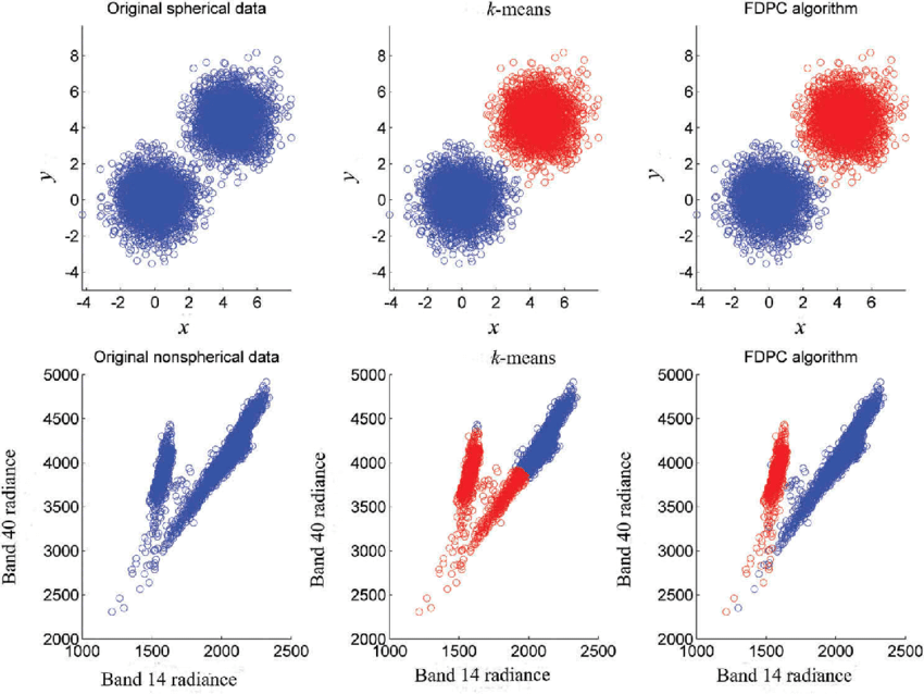
K-Means Clustering algorithms are effective for detecting spherical clusters. Using on datasets with non-spherical clusters can lead to poor clustering results.

K-Means' Focus on Variance $\sigma^2$ and Geometric Interpretation limit its ability to handle non-spherical data, such as that formed in concentric circles or clusters arranged like a rod or a "bean".

Challenges with Non-Spherical Clusters

• Assumption Violation: K-Means prerequisites, including the cluster's spherical shape and equal variance among clusters, aren't met.
• Direct Cost Function Optimization: Minimizing the sum of squared distances impedes the algorithm from conforming to non-spherical shapes.

Visual Reperesentation

Practical Limitations

1. Data Preprocessing: Reshaping the data to be more spherical doesn't always result in the desired clustering.

2. Retrieval Bias: Just because the clusters created by K-Means don't align well with the actual clusters doesn't mean the key centroids aren't hovering around the observable ones.

3. Boundary Ambiguity: When clusters intersect (e.g., two rings where one is nested within the other), it's common for K-Means to struggle to distinguish their respective boundaries.

4. Global Optima Dependence: The algorithm's outcomes are heavily influenced by its initial centroid placement. Confirming non-spherical clusters is trickier if they are concentric, because this dilemma is more pronounced.

Code Example: Visualizing K-Means Limitations

Here is the Python code:

import numpy as np
import matplotlib.pyplot as plt
from sklearn.datasets import make_circles
from sklearn.cluster import KMeans

# Generate non-spherical data
X, _ = make_circles(n_samples=1000, factor=0.5, noise=0.05)

# Fit K-Means
kmeans = KMeans(n_clusters=2, random_state=0).fit(X)

# Visualize the data and K-Means clusters
plt.figure(figsize=(8, 5))
plt.scatter(X[:, 0], X[:, 1], c=kmeans.labels_, cmap='viridis')
plt.scatter(kmeans.cluster_centers_[:, 0], kmeans.cluster_centers_[:, 1], c='red', marker='x', s=100)
plt.title("K-Means in Action on Non-Spherical Data")
plt.show()

In this example, you can use the make_circles function from sklearn.datasets to generate a dataset with non-spherical clusters. After applying K-Means, the displayed plot will demonstrate how the algorithm performs on such data.

13. How do you handle outliers in the K-Means algorithm?

K-Means is sensitive to outliers. These data points can distort cluster boundaries and centroid positions. Here are some strategies in a suggested order of application and considerations for each technique.

Strategies to Handle Outliers in K-Means

1. Pre-Processing Steps

• Data Segmentation: Approach each cluster separately.
• Dimensionality Reduction: Use techniques like Principal Component Analysis (PCA) to identify and eliminate irrelevant dimensions.

2. Outlier Identification Methods

• Statistical Methods: Leverage z-scores or standard deviations.
• Distance-Based: Identify outliers based on their distances from the center.

3. Outlier Handling Methods

• Removal: Exclude detected outliers from clustering.
• Transformation: Use mathematical functions like square root or logarithm to minimize the impact of larger values.

4. Cluster Analysis

Evaluate clusters visually using techniques such as the "elbow method" to determine the number of clusters. Keep in mind that "true" cluster numbers might not be known in advance. Silhouette analysis can also help in identifying a suitable number of clusters.

5. Outsider Labeling

Consider labeling detected outliers post-clustering based on their attributions and characteristics.

6. Advanced Techniques

• Robust Clustering Models: Explore using algorithms like DBSCAN and MeanShift, which are less sensitive to outliers.
• Ensemble Techniques: Combine multiple clusterings to improve robustness.
• Density-Based Models: Implement algorithms like OPTICS to identify spatial outliers.

14. Discuss the concept and importance of feature scaling in K-Means Clustering.

Feature scaling is a critical pre-processing step in K-Means Clustering. The process involves transforming data attributes to a standard scale, improving the performance and interpretability of the clustering algorithm.

The Need for Feature Scaling in K-Means Clustering

• Homogeneity of Feature Importance: K-Means treats all features equally. Scaling makes sure features with larger variances don't disproportionately influence the algorithm.

• Equidistance Assumption: By design, K-Means calculates distances using Euclidean or squared Euclidean metric. These distance metrics become inaccurate without standardized scales.

Feature Scaling Techniques

• Min-Max Scaling: Scales values between 0 and 1.

• Z-Score Normalization: Also known as Standardization, this method scales data to have a mean of 0 and a standard deviation of 1.

• Robust Scaling: Uses interquartile range rather than the mean or variance, making it suitable for data with outliers.

Code Example: Feature Scaling

Here is the Python code:

from sklearn.preprocessing import StandardScaler
from sklearn.cluster import KMeans
import pandas as pd

# Generate some sample data
data = {'X': [18, 22, 35, 60, 75, 85], 'Y': [120, 100, 150, 175, 185, 200]}
df = pd.DataFrame(data)

# Standardize the data using Z-Score
scaler = StandardScaler()
standardized_data = scaler.fit_transform(df)

# Perform K-Means on the standardized data
kmeans = KMeans(n_clusters=2).fit(standardized_data)

15. Why is K-Means Clustering considered a greedy algorithm?

K-Means Clustering is renowned for both its simplicity and effectiveness. However, it is classified as a greedy algorithm, featuring straightforward steps with local and current decision-making criteria.

Core Algorithm Steps

1. Centroid Initialization: Random or heuristic centroid selections.
2. Assignment Stage: Data points are assigned to their nearest cluster center.
3. Update Stage: Cluster centers are moved to the mean of their assigned points.
4. Convergence Check: Iteratively repeats steps 2 and 3 until a stopping criterion is met.

Greedy Characteristics

• Local Optimization: Each step aims at an immediate improvement.

• Lack of Global View: There are no guarantees of finding the best solution.

Influence of Starting Points

The K-Means algorithm's final outcome heavily depends on the initial centroid state, often referred to as the seed selection. Diverse initializations may lead to entirely different cluster configurations.

To mitigate this sensitivity, multiple initializations followed by a selection mechanism (e.g., silhouette score, costs) can provide more robust results. Such methods are frequently implemented in libraries like scikit-learn.

Explore all 50 answers here 👉 Devinterview.io - K-Means Clustering