
You can also find all 45 answers here 👉 Devinterview.io - Probability
Probability serves as the mathematical foundation of Machine Learning, providing a framework to make informed decisions in uncertain environments.
-
Classification: Bayesian methods use prior knowledge and likelihood to classify data into target classes.
-
Regression: Probabilistic models predict distributions over possible outcomes.
-
Clustering: Gaussian Mixture Models (GMMs) assign data points to clusters based on their probability of belonging to each.
-
Modeling Uncertainty: Techniques like Monte Carlo simulations use probability to quantify uncertainty in predictions.
-
Bayesian Inference: Updates the likelihood of a hypothesis based on evidence.
-
Expected Values: Measures the central tendency of a distribution.
-
Variance: Quantifies the spread of a distribution.
-
Covariance: Describes the relationship between two variables.
-
Independence: Variables are independent if knowing the value of one does not affect the probability of the others.
Here is the Python code:
import numpy as np
import matplotlib.pyplot as plt

# Define input data
data = np.array([1, 1, 1, 3, 3, 6, 6, 9, 9, 9])

# Create a probability mass function (PMF) using numpy and the data
def compute_pmf(data):
    unique, counts = np.unique(data, return_counts=True)
    pmf = counts / data.size
    return unique, pmf

# Plot the PMF
def plot_pmf(unique, pmf):
    plt.bar(unique, pmf)
    plt.title('Probability Mass Function')
    plt.xlabel('Unique Values')
    plt.ylabel('Probability')
    plt.show()

unique_values, pmf_values = compute_pmf(data)
plot_pmf(unique_values, pmf_values)In the field of probability, a sample space and an event are foundational concepts, providing the fundamental framework for understanding probabilities.
The sample space, often denoted by
For a random experiment, the sample space is the set of all possible outcomes of that experiment.
Events are subsets of the sample space, defining specific occurrences or non-occurrences based on the outcomes of a random experiment.
Continuing with the coin flip example, let's define two events:
-
$A$ : The coin lands as heads$A = {H}$
-
$B$ : The coin lands as tails$B = {T}$
An event
- An element of the sample space (e.g.,
$H$ for a coin flip). - Represented by a single outcome from the sample space.
- A combination of simple events (e.g., "landing heads and a prime number" for a fair 6-sided die).
- Represented by the union, intersection, or complement of simple events.
In probability theory, a tail event is an event that results from the outcomes of a sequence of independent random variables. Such events often have either very low or high probabilities, making them of particular interest in certain probability distributions, including the Poisson distribution and the Gaussian distribution.
Probability distributions form the backbone of the field of statistics and play a crucial role in machine learning. These distributions characterize the probability of different outcomes for different types of variables.
- Definition: Discrete distributions map to countable, distinct values.
- Example: Binomial Distribution models the number of successes in a fixed number of Bernoulli trials.
- Visual Representation: Discrete distributions are typically represented as bar graphs where each bar represents a specific outcome and its corresponding probability.
-
Probability Function: Discrete distributions have a probability mass function (PMF),
$P(X=k)$ , where$k$ is a specific value.
- Definition: Continuous distributions pertain to uncountable, continuous numerical ranges.
- Example: Normal Distribution represents a wide range of real-valued variables and is frequently encountered in real-world data.
- Visual Representation: Continuous distributions are displayed as smooth, continuous curves in probability density functions (PDFs), with the area under the curve representing probabilities.
-
Probability Function: Continuous distributions use the PDF,
$p(x)$ . The probability within an interval is given by the integral of the PDF across that interval, i.e.,$P(a \leq X \leq b) = \int_{a}^{b} p(x) , dx$ .
- Discrete Distributions: Discrete distributions are commonly found in datasets with distinct, countable outcomes. A classic example is survey data where responses are often in discrete categories.
- Continuous Distributions: Real-world numerical data, such as age, height, or weight, often follows a continuous distribution.
Joint probabilities quantify the likelihood of multiple events occurring simultaneously.
Marginal probabilities, derived from joint probabilities, represent the likelihood of individual events.
Conditional probabilities describe how the likelihood of one event changes given knowledge of another event.
-
Joint Probability: P(A \cap B)
-
Marginal Probability: P(A) or P(B)
-
Conditional Probability: P(A|B) or P(B|A)
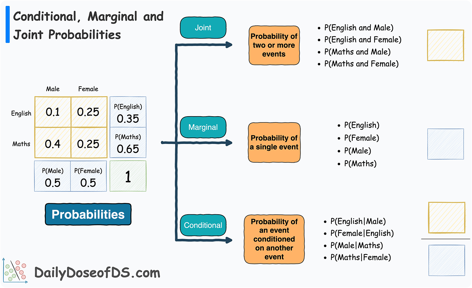
The conditional probability of event A given event B is calculated using the following formula:
Marginal probabilities are obtained by summing (in the case of two variables, like X and Y) or integrating (in the case of continuous variables or more than two variables) the joint probabilities over the events not involved in the marginal probability. In the case of two variables X and Y, the marginal probability can be calculated as follows:
Independence in the context of probability refers to two or more events' behaviors where the occurrence (or non-occurrence) of one event does not affect the probability of the other(s).
-
Mutual Exclusivity: If both events cannot occur at the same time,
$P(A \text{ and } B) = 0$ . -
Conditional Independence: When the occurrence of a third event sets two others as independent only under this particular condition. This is mathematically expressed as
$P(A \text{ and } B | C) = P(A|C) \times P(B|C)$ .
Two events,
The formula
-
Inexhaustibility: Independence doesn't infer that the combined probability
$P(A \text{ and } B)$ necessarily equals$1$ . Events can be independent and still have a joint probability less than$1$ .
Bayes' Theorem is a fundamental concept in probability theory that allows you to update your beliefs about an event based on new evidence.
The probability of an event, given some evidence, is calculated as follows:
Where:
-
$P(A|B)$ is the posterior probability of$A$ given$B$ -
$P(B|A)$ is the likelihood of$B$ given$A$ -
$P(A)$ is the prior probability of$A$ -
$P(B)$ is the total probability of$B$
Consider a doctor using a diagnostic test for a rare disease. If the disease is present, the test is positive
Without considering the test accuracy and base rate, one might calculate the probability of having the disease given a positive test
This calculation, however, neglects the reality that the disease is rare.
To find the true probability using Bayes' Theorem, we break it down as:
Where:
-
$P(+|D) = 0.99$ is the probability of a positive test given the disease -
$P(D) = 0.01$ is the prior probability of having the disease -
$P(+)$ is the total probability of a positive test and can be calculated using the Law of Total Probability:
Substituting in the given values:
So,
This means that even with a positive test result, the probability of having the disease is less than 50% due to the test's false-positive rate and the disease's low prevalence.
A probability density function (PDF) characterizes the probability distribution of a continuous random variable
The PDF expresses the relative likelihood of
-
Non-negative over the entire range:
$f(x) ≥ 0$ - Area under the curve: The integral of the PDF over the entire range equals 1.
-
Cumulative Density Function (CDF): Represents the probability that
$X$ takes a value less than or equal to$x$ .
Mathematically, the CDF is obtained by integrating the PDF from
- Expected Value: Also known as the mean of the distribution, it gives the center of "gravity" of the PDF.
For continuous random variables:
The normal distribution describes many natural phenomena and often serves as a first approximation for any unknown distribution.
Its PDF is given by the mathematical expression:
Where:
-
$\mu$ represents the mean. -
$\sigma^2$ serves as the variance, controlling the distribution's width. The square root of the variance yields the standard deviation$\sigma$ .
The Cumulative Distribution Function (CDF) provides valuable insights in both discrete and continuous probability distributions by characterizing the probability distribution of a random variable. By evaluating the CDF at a given point, we can determine the probability that the random variable is below (or equal to) that point.
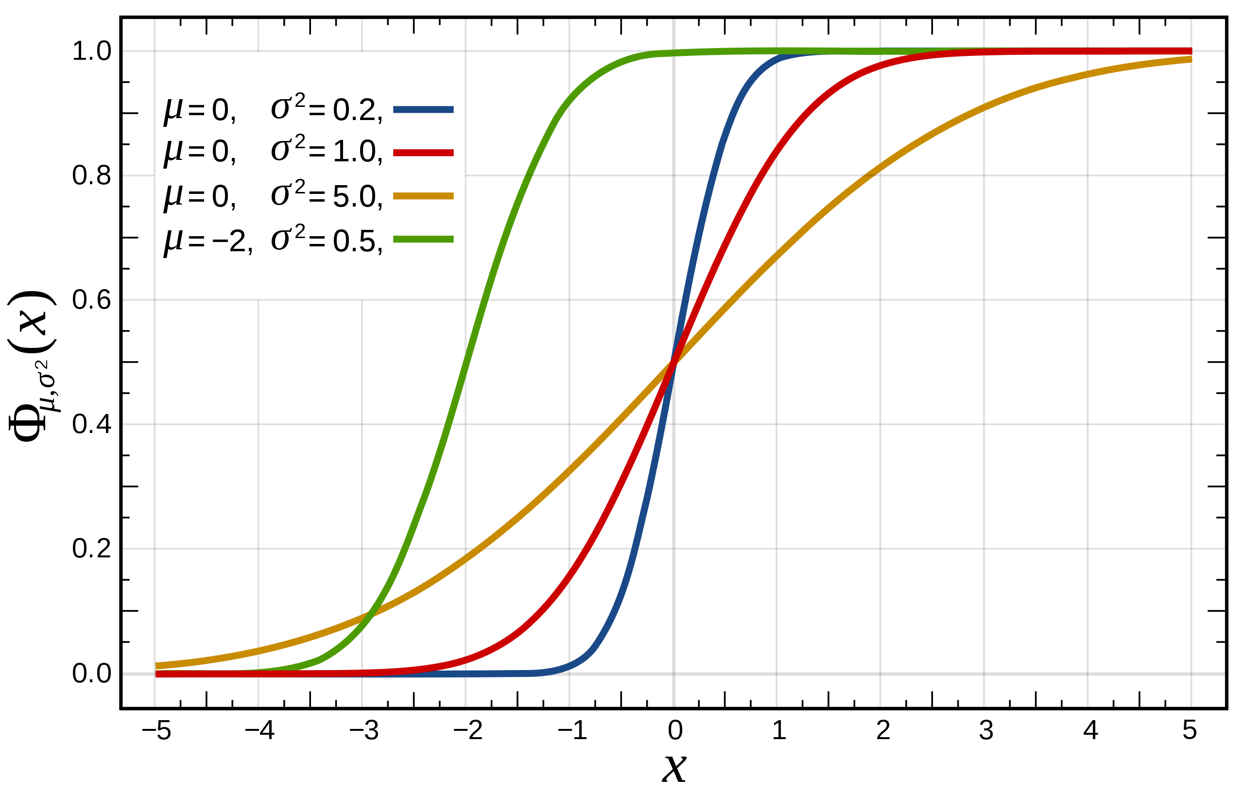
- Visualizing and Understanding Distributions: The CDF is beneficial for exploring datasets, as it offers a graphical portrayal of data distributions, allowing for quick inferences about characteristic features.
- Quantifying the Likelihood of Outcomes: Once the CDF is known, it becomes straightforward to compute probabilities for specific outcomes.
- Monotonicity: The CDF is a monotonically increasing function. As the input value increases, so do the output values.
-
Bounds: For any real number, the CDF value falls between
$0$ and$1$ . - Characterizing the Distribution: The CDF is the official standard for unraveling any probability distributions, with its form, either explicit or implicit, catering to that particular goal.
While the exact form of a CDF can be complex, numerical techniques and quantiles offer straightforward methods for evaluation and interpretation.
For a random variable
where the integral may be replaced by a summation in the case of discrete distributions.
The CDF is given by:
where
The Central Limit Theorem (CLT) serves as a foundational pillar for statistical inference and its implications are widespread across machine learning and beyond.
The CLT states that given a sufficiently large sample size from a population with a finite variance, the distribution of the sample means will converge to a normal distribution, regardless of the shape of the original population distribution.
In mathematical terms, if we have a sample of
Below is an example illustrating the transformation of a non-normally distributed dataset to one that adheres to a normal distribution as the sample size increases:
The Central Limit Theorem is Intricately woven into various areas of machine learning:
-
Parameter Estimation: It makes possible point estimation techniques like maximum likelihood estimation and confidence interval estimation.
-
Hypothesis Testing: It underpins many classical statistical tests, such as the Z-test and t-test to evaluate the significance of the sample data.
-
Model Evaluation Metrics: It validates the use of metrics like the mean and variance across cross-validations, boosting the reliability of model assessments.
-
Error Distributions: It justifies the assumption of normally distributed errors in several regression techniques.
-
Algorithm Design: Many iterative algorithms, like EM algorithm and stochastic gradient descent, leverage the concept to refine their estimations.
-
Ensemble Methods: Techniques like bagging (Bootstrap Aggregating) and stacking exploit the theorem, further enriching prediction accuracy.
The Law of Large Numbers (LLN) represents an essential statistical principle. It states that as the size of a sample or dataset increases, the sample mean will tend to get closer to the population mean.
In an experiment with independent and identically distributed (i.i.d) random variables, the LLN assures convergence in probability. This implies that the probability of the sample mean differing from the true mean by a certain threshold reduces as the sample size grows.
Let
According to the Weak Law of Large Numbers (WLLN), the sample mean
In other words, the probability that the sample mean deviates from the population mean by more than
- Sample Size Significance: It underscores the need for sufficiently large sample sizes in statistical studies.
- Survey Accuracy: Larger survey data generally provides more reliable insights.
- Financial Forcasting: Greater historical data can lead to more accurate estimates in finance.
- Risk Assessment: More data can enhance the precision in evaluating potential risks.
Here is the Python code:
import numpy as np
import matplotlib.pyplot as plt

np.random.seed(0)

# Generate random data from a standard normal distribution
data = np.random.randn(1000)

# Calculate the running sample mean
running_mean = np.cumsum(data) / (np.arange(1, 1001))

# Plot the running sample means
plt.plot(running_mean, label='Running Sample Mean')
plt.axhline(np.mean(data), color='r', linestyle='--', label='True Mean')
plt.xlabel('Sample Size')
plt.ylabel('Mean')
plt.legend()
plt.show()Expectation, variance, and covariance are fundamental mathematical concepts pertinent to understanding probability distributions.
The expectation, represented as
It is calculated by the weighted sum of all possible outcomes, where the weights are given by the probability of each outcome,
In a continuous setting, the sum is replaced by an integral:
where
The variance, denoted as
It is calculated as the expected value of the squared deviation from the mean:
where
The covariance, symbolized as
Mathematically, given two random variables
In terms of their joint probability,
An alternative formula based on the definitions of expectation is:
where
The Kronecker delta function
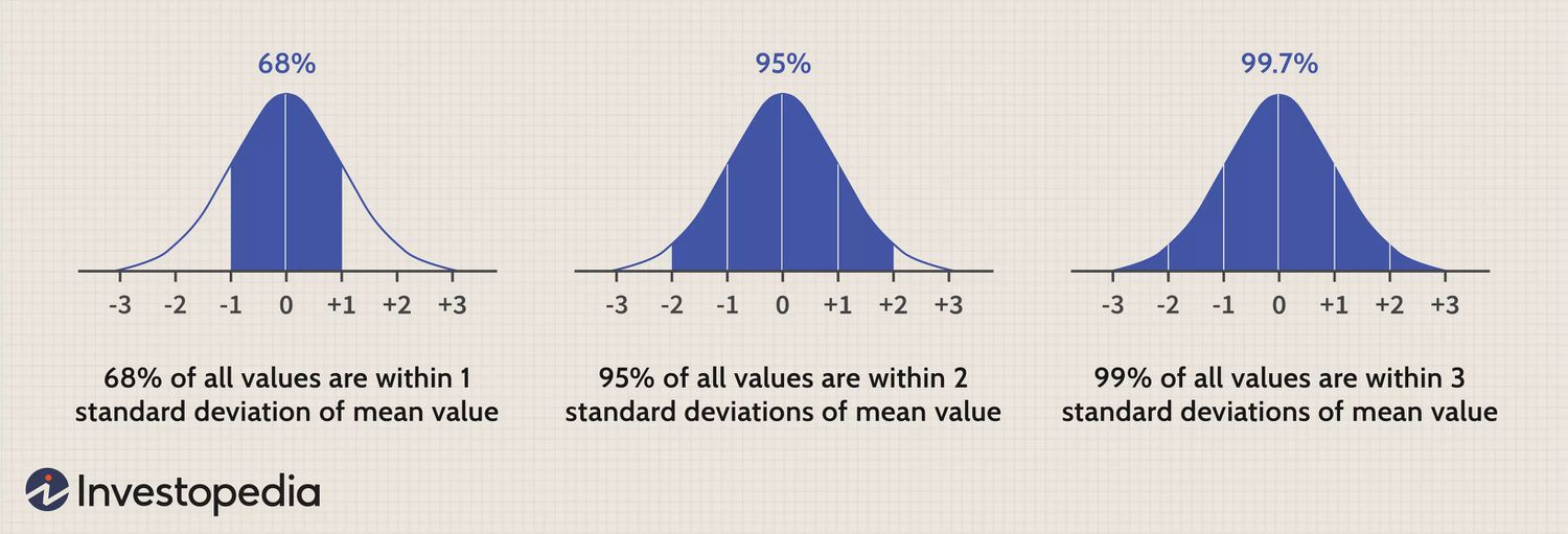
The Gaussian distribution, also known as the Normal distribution, is a key concept in probability and statistics. Its defining characteristic is its bell-shaped curve, which provides a natural way to model many real-world phenomena.
-
Location and Spread: Described by parameters
$\mu$ (mean) and$\sigma$ (standard deviation), the Gaussian distribution is often centered around its mean, with fast decays in the tails. -
Symmetry: The distribution is symmetric around its mean. The area under the curve is 1, representing the totality of possible outcomes.
-
Inflection Points: The points of maximum curvature, known as inflection points, lie
$\pm \sigma$ from the mean. -
Standard Normal Form: A Gaussian with
$\mu = 0$ and$\sigma = 1$ is in its standard form. -
Empirical Rule: This rule states that for any Gaussian distribution, about 68% of the data lies within
$\pm 1$ standard deviation, 95% within$\pm 2$ standard deviations, and 99.7% within$\pm 3$ standard deviations of the mean.
The probability density function (PDF) for a Gaussian distribution is:
Where:
-
$x$ represents a specific value or observation -
$\mu$ is the mean -
$\sigma$ is the standard deviation

In the context of the Empirical Rule, notice the intervals of $\mu \pm \sigma, \mu \pm 2\sigma,$and
Numerous natural systems exhibit behavior that aligns with a Gaussian distribution, including:
- Human Characteristics: Variables such as height, weight, and intelligence often conform to a Gaussian distribution.
- Biological Processes: Biological phenomena, such as heart rate variability and the duration of animal movements, are frequently governed by the Gaussian distribution.
- Environmental Events: Natural occurrences such as floods, rainfall, and wind speed in many regions adhere to a Gaussian model.
The Gaussian Distribution proves equally valuable in artificial systems, from finance to machine learning, owing to its mathematical elegance and widespread applicability.
The Binomial Distribution is a key probability distribution in machine learning and statistics. It models the number of successes in a fixed number of independent Bernoulli trials.
-
Classification: In a binary classifier, each example is a Bernoulli event; the binomial distribution helps estimate the number of correct predictions within a set.
-
Feature Selection: Assessing the significance of a feature in a dataset can be done in binary settings, where we calculate if the resulting classes are distributed in a manner not compatible with a 50-50 division.
-
Model Evaluation Metrics: Binomial calculations are behind widely used model evaluation metrics like accuracy, precision, recall, and F1 scores.
-
Ensemble Learning: Techniques like Bagging and Random Forest involve numerous bootstrap samples, essentially Bernoulli trials, to build diverse classifiers resulting from resampling methods.
-
Hyperparameter Tuning: Algorithms like Grid Search or Random Search often rely on cross-validated performance measures exhibiting a binomial nature.
-
Quality Assurance: Determine the probability of a machine learning-based quality control mechanism correctly identifying faulty items.
-
A/B Testing: Analyzing user responses to two different versions of a product, such as a website or an app.
-
Revenue Prediction: Predicting customer behavior, such as converting to a paid subscription, based on historical data.
-
Anomaly Detection: Identifying unusual patterns in data, such as fraudulent transactions in finance.
-
Performance Monitoring: Evaluating the reliability of systems or their components.
-
Risk Management: Estimating and managing various types of risks in business or financial domains.
-
Medical Diagnosis: Assessing the performance of diagnostic systems in identifying diseases or conditions.
-
Weather Forecasting: Identifying extreme weather occurrences from historical patterns.
-
Voting Behavior Analysis: Assessing the likelihood of an event, like winning an election, based on survey results.
Both the Poisson and the Binomial distributions relate to counts, but they're applied in different settings and have key distinctions.
- Nature of the Variable: The Poisson distribution is used for counts of rare events that occur in a fixed time or space interval, while the Binomial distribution models the number of successful events in a fixed number of trials.
-
Number of Trials: The Poisson distribution assumes an infinite number of trials, while the Binomial distribution has a fixed, finite number of trials,
$n$ . -
Probability of Success: In the Binomial distribution,
$p$ remains constant across trials, representing the probability of a success. In the Poisson,$p$ becomes infinitesimally small as$n$ becomes large to approximate a rare event.
Both distributions deal with discrete random variables and are characterized by a single parameter:
-
Poisson Distribution: The single parameter,
$\mu$ , denotes the average rate of occurrence for the event. -
Binomial Distribution: The single parameter,
$n$ the number of trials, and$p$ the probability of success on each trial, together determine the shape of the distribution.
The probability mass function (PMF) of the Poisson distribution is defined as:
Where:
-
$k$ is the count of events that occurred in the fixed interval. -
$\mu$ is the average rate at which events occur in that interval, also known as the Poisson parameter. -
$e$ is Euler's number, approximately 2.71828.
The probability mass function (PMF) of the Binomial distribution is defined as:
Where:
-
$k$ is the number of successful events. -
$n$ is the total number of independent trials. -
$p$ is the probability of success on each trial.
The shape of the Poisson distribution is unimodal, with the PMF reaching its maximum at

The Binomial distribution is less smooth and can be symmetric or skewed, depending on the value of

Bernoulli distribution is foundational to probabilistic models, including some key techniques in Machine Learning, such as Naive Bayes and various binary classification algorithms.
-
Binary Outcomes: The Bernoulli distribution describes the probability of success or failure when
$n = 1$ . For instance, in Binary Classification, where there are only two possible outcomes:$y \in \left\lbrace 0, 1 \right\rbrace$ . -
Probabilistic Classification: In binary classification, the model estimates the probability of a sample belonging to the positive class. This estimate stems from the Bernoulli distribution.
-
Independence Assumption: Some models, like Naive Bayes, assume feature independence, simplifying the joint probability into a product of individual ones. Each feature is then modeled using a separate Bernoulli distribution.
The Bernoulli distribution is employed in numerous real-world contexts, enabled by its implementation in diverse Machine Learning projects. Common domains include Natural Language Processing, Image Segmentation, and Medical Diagnosis.
Here is the Python code:
from sklearn.naive_bayes import BernoulliNB
import numpy as np

# Binary features
X = np.random.randint(2, size=(100, 3))
y = np.random.randint(2, size=100)

# Multinomial Naive Bayes
clf = BernoulliNB()
clf.fit(X, y)
Explore all 45 answers here 👉 Devinterview.io - Probability