Devinterview-io/sql-ml-interview-questions

🟣 SQL interview questions and answers to help you prepare for your next machine learning and data science interview in 2025.

55 Fundamental SQL in Machine Learning Interview Questions

You can also find all 55 answers here 👉 Devinterview.io - SQL

1. What are the different types of JOIN operations in SQL?

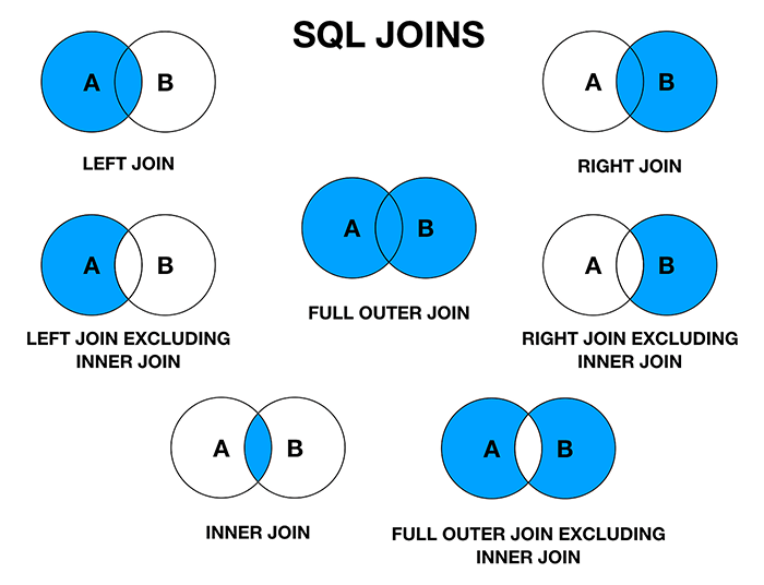
INNER JOIN, LEFT JOIN, RIGHT JOIN, and FULL JOIN are different SQL join types, each with its distinct characteristics.

Join Types at a Glance

• INNER JOIN: Returns matching records from both tables.
• LEFT JOIN: Retrieves all records from the left table and matching ones from the right.
• RIGHT JOIN: Gets all records from the right table and matching ones from the left.
• FULL JOIN: Includes all records when there is a match in either of the tables.

Visual Representation

Code Example: SQL Joins

Here is the SQL code:

-- CREATE TABLES
CREATE TABLE employees (
    id INT PRIMARY KEY,
    name VARCHAR(100),
    department_id INT
);

CREATE TABLE departments (
    id INT PRIMARY KEY,
    name VARCHAR(100)
);

-- INSERT SOME DATA
INSERT INTO employees (id, name, department_id) VALUES
  (1, 'John', 1), 
  (2, 'Alex', 2), 
  (3, 'Lisa', 1), 
  (4, 'Mia', 1);

INSERT INTO departments (id, name) VALUES 
  (1, 'HR'), 
  (2, 'Finance'), 
  (3, 'IT');

-- INNER JOIN
SELECT employees.name, departments.name as department
FROM employees
INNER JOIN departments ON employees.department_id = departments.id;

-- LEFT JOIN
SELECT employees.name, departments.name as department
FROM employees
LEFT JOIN departments ON employees.department_id = departments.id;

-- RIGHT JOIN
SELECT employees.name, departments.name as department
FROM employees
RIGHT JOIN departments ON employees.department_id = departments.id;

-- FULL JOIN
SELECT employees.name, departments.name as department
FROM employees
FULL JOIN departments ON employees.department_id = departments.id;

2. Explain the difference between WHERE and HAVING clauses.

The WHERE and HAVING clauses are both used in SQL, but they serve distinct purposes,

Key Distinctions

• WHERE: Filters records based on conditions for individual rows.
• HAVING: Filters the results of aggregate functions, such as COUNT, SUM, AVG, and others, for groups of rows defined by the GROUP BY clause.

Code Example: Basic Usage

Here is the SQL code:

-- WHERE: Simple data filtering
SELECT product_type, AVG(product_price) AS avg_price
FROM products
WHERE product_price > 100
GROUP BY product_type;

-- HAVING: Filtered results post-aggregation
SELECT order_id, SUM(order_total) AS total_amount
FROM orders
GROUP BY order_id
HAVING SUM(order_total) > 1000;

3. How would you write a SQL query to select distinct values from a column?

When you have duplicates in a column, you can use the DISTINCT clause to retrieved unique values.

For instance:

SELECT UNIQUE_COLUMN
FROM YOUR_TABLE
ORDER BY UNIQUE_COLUMN;

In this query, replace UNIQUE_COLUMN with the column name from which you want distinct values, and YOUR_TABLE with your specific table name.

Practical Example: Using DISTINCT

Let's say you have a table students_info with a grade column indicating the grade level of students. You want to find all unique grade levels.

Here's the corresponding SQL query:

SELECT DISTINCT grade
FROM students_info
ORDER BY grade;

Executing this query would return a list of unique grade levels in ascending order.

When to Use DISTINCT

• Unique Records: When you only want to see and count unique values within a specific column or set of columns.

  SELECT COUNT(DISTINCT column_name) FROM table_name;

• Criteria Comparison: Using IN and NOT IN can involve multiple selections; DISTINCT ensures the return of unique results.

• Insight into Overlapping Data: Useful for data analysis tasks where you want to identify shared information between rows.

• Subset Selection: When you are working with large tables and want to zero in on unique records within a specific range, such as for pagination.

4. What does GROUP BY do in a SQL query?

GROUP BY is a powerful clause in Structured Query Language (SQL) that allows for data summarization and grouping.

Key Functions

• Aggregation: Performs tasks like sum, count, average, among others within subsets (groups).
• Grouping: Identifies data subsets based on predetermined commonalities.
• Filtering: Enables filtering both pre- and post-aggregation.

When to Use GROUP BY

• Summarizing Data: For instance, calculating a 'Total Sales' from individual transactions.
• Categorization: Such as counting the number of 'Customers' or 'Products' within specific groups (like regions or categories).
• Data Integrity Checks: To identify potential duplicates or check for data consistency.
• Combining with Aggregate Functions: Pairing with functions such as COUNT, SUM, AVG, MAX, and MIN for more sophisticated calculations.

The Mechanism Behind GROUP BY

• Division into Groups: The system sorts the result set by the specified columns in the GROUP BY clause and groups rows that have the same group column values. This step creates a distinct group for each unique combination of 'group by' columns.
• Aggregation within Groups: The system then applies the aggregation function (or functions) to each group independently, summarizing the data within each group.
• Result Generation: After the groups are processed, the final result set is produced.

Code Example: GROUP BY in Action

Here is the SQL code:

SELECT SUM(Revenue), Region
FROM Sales
GROUP BY Region;

In this example, the Sales table is grouped by Region, and the sum of Revenue is calculated for each group.

Potential Challenges with GROUP BY

• Single-Column Limitation: Without employing additional techniques, such as using subqueries or rollup or cube extensions, data can be grouped on only one column.
• Data Types Consideration: When grouping by certain data types, such as dates or floating points, results may not be as expected due to inherent characteristics of those types.

Advanced Techniques with GROUP BY

• Rollup and Cube: Extensions providing multi-level summaries.

  • ROLLUP: Computes higher-level subtotals, moving from right to left in the grouping columns.
  • CUBE: Computes all possible subtotals.

• Grouping Sets: Defines multiple groups in one query, e.g., grouping by year, month, and day in a date column.

5. How can you aggregate data in SQL (e.g., COUNT, AVG, SUM, MAX, MIN)?

Aggregating data in SQL is essential for making sense of large data sets. Common aggregate functions include COUNT, SUM, AVG (mean), MIN, and MAX.

Syntax

Here is an example of the SQL code:

SELECT AGG_FUNCTION(column_name)
FROM table_name
GROUP BY column_name;

• AGG_FUNCTION: Replace with any of the aggregate operations.
• column_name: The specific column to which the function will be applied.

If you don't use a GROUP BY clause, the query will apply the aggregate function to the entire result set.

Examples

Without GROUP BY

SELECT COUNT(id) AS num_orders
FROM orders;

With GROUP BY

SELECT customer_id, COUNT(id) AS num_orders
FROM orders
GROUP BY customer_id;

In this example, the COUNT aggregates the number of orders for each unique customer ID.

Considerations

• Null Values: Most aggregates ignore nulls, but you can use COUNT(*) to include them.
• Multiple Functions: It's possible to include multiple aggregate functions in one query.
• Data Type Compatibility: Ensure that the chosen aggregate function is compatible with the data type of the selected column. For instance, you can't calculate the mean of a text field.

Code Example: Aggregating Data in SQL

Here is the SQL code:

CREATE TABLE orders (id INT, customer_id INT, total_amount DECIMAL(10, 2));

INSERT INTO orders (id, customer_id, total_amount)
VALUES 
	(1, 101, 25.00),
	(2, 102, 35.50),
	(3, 101, 42.25),
	(4, 103, 20.75),
	(5, 102, 60.00);

-- Total Number of Orders
SELECT COUNT(id) AS num_orders
FROM orders;

-- Number of Orders per Customer
SELECT customer_id, COUNT(id) AS num_orders
FROM orders
GROUP BY customer_id;

-- Total Sales
SELECT SUM(total_amount) AS total_sales
FROM orders;

-- Average Order Value
SELECT AVG(total_amount) AS avg_order_value
FROM orders;

-- Highest Ordered Value
SELECT MAX(total_amount) AS max_order_value
FROM orders;

-- Lowest Ordered Value
SELECT MIN(total_amount) AS min_order_value
FROM orders;

6. Describe a subquery and its typical use case.

A subquery consists of a complete SQL statement nested within another query. It's often used for complex filtering, calculations, and data retrieval.

Subqueries are broadly classified into two types:

• Correlated: They depend on the outer query's results. Each time the outer query iterates, the subquery is re-evaluated with the updated outer result. It can be less efficient as it often involves repeated subquery evaluation.
• Uncorrelated: These are self-contained and don't rely on the outer query. They are typically executed only once and their result is used throughout the outer query.

Common Use Cases

• Filtering with Aggregates: Subqueries can be used in combination with aggregate functions to filter group-level results based on specific criteria. For instance, you can retrieve departments with an average salary above a certain threshold.

• Multi-Criteria Filtering: Subqueries are often handy when traditional WHERE, IN, or EXISTS clauses can't accommodate complex, multi-criteria filters.

• Data Integrity Checks: Subqueries can help identify inconsistent data by comparing values to related tables.

• Hierarchical Data Queries: With the advent of Common Table Expressions (CTEs) and recursive queries in modern SQL standards, a direct use of subqueries for hierarchical data searches is now uncommon - CTEs are the preferred means of such queries.

• Data Retention: Subqueries can be used to identify specific records to be deleted or retained based on certain conditions.

Common Use Cases

Multi-Criteria Filtering

• Task: Return all customers from a specific city who have placed orders within the last month.
• Code: sql SELECT * FROM Customers WHERE City = 'London' AND CustomerID IN (SELECT CustomerID FROM Orders WHERE OrderDate > DATEADD(month, -1, GETDATE()))

Data Integrity Checks

• Task: Retrieve customers with inconsistent states in the Customer and Order tables.
• Code: sql SELECT * FROM Customer WHERE State NOT IN (SELECT DISTINCT State FROM Orders)

Data Retention

• Task: Archive orders older than three years.
• Code: sql DELETE FROM Orders WHERE OrderID IN (SELECT OrderID FROM Orders WHERE OrderDate < DATEADD(year, -3, GETDATE()))

7. Can you explain the use of indexes in databases and how they relate to Machine Learning?

Database indexes enable systems to retrieve data more efficiently by offering a faster look-up mechanism. This optimization technique is directly pertinent to Machine Learning.

Indexes in Databases

Databases traditionally use B-Tree indexes, but are equipped with several index types, catering to varying data environments and query patterns.

• B-Tree (Balanced Tree): Offers balanced search capabilities, ensuring nodes are at least half-full.
• Hash: Employed for point queries, dedicating fixed-size chunks to keys.
• Bitmap: Particularly suitable for low-cardinality data where keys are better represented as bits.
• Text Search: Facilitates efficient text matching.

Key Concepts of B-Trees

• Node Structure: Contains keys and pointers. Leaf nodes harbor actual data, enabling direct access.
• Data Positioning: Organizes data in a sorted, multi-level structure to expedite lookups.
• Range Queries: Suited for both singular and range-based queries.

Machine Learning Query Scenarios

• Similarity Look-Up: A dataset with user preferences can be indexed to expedite locating individuals with matching profiles, advantageous in applications such as recommendation systems.
• Range-Based Searches: For datasets containing time-specific information, like a sales record, B-Trees excel in furnishing time-ordered data within designated intervals.

Code Example: Implementing B-Trees for Range Queries

Here is the Python code:

class Node:
    def __init__(self, keys=[], children=[]):
        self.keys = keys
        self.children = children

# Perform range query on tree rooted at 'node'
def range_query(node, start, end):
    # Base case: Leaf node
    if not node.children:
        return [key for key in node.keys if start <= key <= end]
    # Locate appropriate child node
    index = next((i for i, key in enumerate(node.keys) if key >= start), len(node.children) - 1)
    return range_query(node.children[index], start, end)

8. How would you optimize a SQL query that seems to be running slowly?

When a SQL query is sluggish, various optimization techniques can be employed to enhance its speed. Let's focus on the logical and physical design aspects of the database structure and the query itself.

Key Optimization Techniques

1. Query Optimization

• Simplify Complex Queries: Break the query into smaller parts for better readability and performance. Use common table expressions or derived tables to modularize SQL logic. Alternatively, you can use temporary tables.
• Limit Result Set: Use TOP, LIMIT, or ROWNUM/ROWID to restrict the number of records returned.
• Reduce JOIN Complexity: Replace multiple JOINs with fewer, multi-table JOINs and explicit JOIN notation.

2. Indexing

• Proper Indexing: Select suitable columns for indexing to speed up data retrieval. Use composite indexes for frequent combinations of columns in WHERE or JOIN conditions.
• Avoid Over-Indexing: Numerous indexes can slow down write operations and data modifications. Strike a balance.

3. Schema and Data Design

• Normalization: Ensure the database is in an optimal normal form, which can reduce redundancy, maintain data integrity, and minimize disk space.
• Data Types: Use appropriate data types for columns to conserve space and support efficient data operations.

4. Under The Hood: The Query Plan

• Analyze Query Execution Plan: Look at the query execution plan, generated by the SQL query optimizer, to identify bottlenecks and improve them. Many RDBMS provide commands and tools to access the query execution plan.

5. More Ideas from SQL Performance Tuning

• Test Under Load: Simulate the production environment and monitor query response times to identify performance issues.
• Limit Data Reallocations in tempdb: Data reallocation operations such as INSERT INTO.. SELECT FROM can be resource-intensive on tempdb.
• Partition Data: Split large tables into smaller, more manageable segments to speed up query performance.

Tools and Techniques for Query Analysis

• Profiling Tools: Use graphical query builders and visual execution plan tools provided by much RDBMS to examine data flow and performance.
• Query Plan Viewer: Databases such as SQL Server have a graphical representation of query execution plans.
• Index Analysis: Some databases, like MySQL and SQL Server, provide tools to check the efficiency of indexes and suggest index changes through Index Tuning Wizard and Optimizer Index Advisor.

Practical Steps for Query Optimization

1. Determine the Performance Problem: Understand what specific aspect of the query is underperforming.
2. Profile Your Query: Use EXPLAIN (or its equivalent on other databases) to see the query plan and identify potential bottlenecks.
3. Analyze Query Execution Time: Use database tools to analyze real execution time and get insights into I/O, CPU, and memory usage.
4. Identify the Bottleneck: Focus on the slowest part of the query or most resource-intensive part, for example, I/O or CPU.
5. Tune That Portion: Make changes to the query or the table structure or consider using versioned views or indexed views. Take time to understand the reason it is being slow and focus your efforts on correcting that.

9. How do you handle missing values in a SQL dataset?

Handling missing values is crucial for accurate analysis in SQL. Let's look at the various techniques for managing them.

Removing Records

One of the simplest ways to deal with missing values is to discard rows with NULLs.

Examples

Here's a SQL query that deletes rows containing NULL in the column age:

DELETE FROM students
WHERE age IS NULL;

Direct Replacement

Replace missing values with specific defaults using COALESCE or CASE statements.

Examples

If grade can have NULL values and you want to treat them as "ungraded":

SELECT student_name, COALESCE(grade, 'Ungraded') AS actual_grade
FROM student_grades;

An example using CASE:

SELECT book_title,
       CASE WHEN publication_year IS NULL THEN 'Unknown'
            ELSE publication_year
       END AS year
FROM books;

Using Aggregates

Apply SQL aggregate functions to compute statistics without explicitly removing NULLs. For example, COUNT ignores NULLs on a column.

SELECT department, COUNT(*) AS total_students
FROM students
GROUP BY department;

Flexible Joins

Depending on your specific situation, you might want to include or exclude missing values when joining tables.

Examples

Using LEFT JOIN:

SELECT s.student_id, s.name, e.enrollment_date
FROM students s
LEFT JOIN enrollments e ON s.student_id = e.student_id;

Using INNER JOIN:

SELECT s.student_id, s.name, e.enrollment_date
FROM students s
INNER JOIN enrollments e ON s.student_id = e.student_id
WHERE e.enrollment_date IS NOT NULL;

Handle Missing Date Fields

If Date fields are missing, the appropriate strategy would depend on the context.

1. Replace with Defaults: For missing dates, you can use a default, such as the current date, or another specific date.

2. Remove or Flag: Another option, based on context, is to either delete the record with the missing date or flag it for later review.

Examples

For replacing with the current date:

SELECT action_id, COALESCE(action_date, CURRENT_DATE) AS actual_date
FROM actions;

3. Impute from Adjacent Data: In time series data, it's often useful to fill in missing dates with the nearest available data point to maintain a continuous date sequence. This can be done using window functions.

Examples

Using LAG() to fill missing dates with the previous non-missing date:

SELECT action_id,
       COALESCE(action_date, LAG(action_date) OVER (ORDER BY action_id)) AS imputed_date
FROM actions;

Advanced Techniques

1. Using Temp Tables: You can create a temporary table, excluding rows with NULLs, and then work with this cleaner dataset.

Example:

CREATE TEMPORARY TABLE clean_students AS
SELECT *
FROM students
WHERE age IS NOT NULL;

-- Perform further tasks using "clean_students" table

2. Machine Learning Methods: Advanced SQL engines supporting ML functionalities might offer methods like imputation based on models.

3. Dynamic Imputation: For scenarios involving complex rules or sequences, you might consider using stored procedures to dynamically impute missing values.

10. Write a SQL query that joins two tables and retrieves only the rows with matching keys.

Problem Statement

The task is to perform a SQL join operation between two tables and retrieve the rows where the keys match.

Solution

To accomplish this task, use the following SQL query.

MySQL

SELECT * 
FROM table1
INNER JOIN table2 ON table1.key = table2.key;

PostgreSQL

SELECT * 
FROM table1
INNER JOIN table2 USING (key);

Oracle

SELECT *
FROM table1
JOIN table2 ON table1.key = table2.key;

SQL Server

SELECT *
FROM table1
JOIN table2 ON table1.key = table2.key;

Key Points

• INNER JOIN: Retrieves the matching rows from both tables based on the specified condition.
• ON, USING: Specifies the column(s) used for joining.
• SELECT: You can specify individual columns instead of * based on requirement.
• Table Aliases: When dealing with long table names, aliases (e.g., t1, t2) provide a more concise syntax.

11. How would you merge multiple result sets in SQL without duplicates?

When you need to combine the result sets of multiple SELECT queries without duplicates, use the UNION set operator. If you want to include duplicates, you can use UNION ALL.

Here is a visual representation of how these set operations work:

Code Example: Using UNION

Here is some SQL code:

SELECT employee_id 
FROM full_time_employees 

UNION 

SELECT intern_id 
FROM interns;

This code retrieves a combined list of unique employee IDs from both full_time_employees and interns tables.

12. Create a SQL query to pivot a table transforming rows into columns.

Problem Statement

"Pivoting" a table in SQL is the process of reorganizing and transforming row data into columnar data, commonly used for reporting or data analysis.

Solution

Two methods for pivoting data in SQL are:

1. Static Pivot: When the distinct values of the pivoted column are known in advance.
2. Dynamic Pivot: When the distinct values are not known in advance and need to be determined at runtime.

Key Considerations

• Pivot Column Values: Aware vs. Unaware of distinct values.
• Performance Impact: Dynamic pivoting often involves complex operations at runtime.
• SQL Compatibility: Dynamic pivoting can be limited in certain SQL dialects.

Here is an example table named salesdata:

Date	Product	Quantity	Amount
1/1/2020	Apples	10	50
1/1/2020	Oranges	8	40
2/1/2020	Apples	12	60
2/1/2020	Oranges	15	75

Static Pivot

The PIVOT keyword is used in SQL Server, and crosstab() is used in PostgreSQL.

Implementing Static Pivot

PostgreSQL:

SELECT *
FROM crosstab(
  'SELECT date, amount, product FROM salesdata ORDER BY 1,3',
  'SELECT DISTINCT product FROM salesdata ORDER BY 1'
) AS ct ("Date" date, "Apples" int, "Oranges" int);

SQL Server:

SELECT *
FROM (SELECT Date, Product, Amount
      FROM salesdata) AS SourceTable
PIVOT (SUM(Amount) FOR Product IN ([Apples], [Oranges])) AS PivotTable;

Dynamic Pivot

For SQL Server, a stored procedure is necessary, as it dynamically constructs the query based on the distinct values.

Implementing Dynamic Pivot

SQL Server:

• Create a stored procedure:

CREATE PROCEDURE dynamicPivot
AS
BEGIN
  DECLARE @cols AS NVARCHAR(MAX), @query AS NVARCHAR(MAX);
  SELECT @cols = STUFF((SELECT DISTINCT ',' + QUOTENAME(Product) FROM salesdata FOR XML PATH('')), 1, 1, '');
  SET @query = 'SELECT Date, ' + @cols + ' FROM (SELECT Date, Product, Amount FROM salesdata) AS SourceTable PIVOT (SUM(Amount) FOR Product IN (' + @cols + ' )) AS PivotTable;';
  EXEC sp_executesql @query;
END;

• Execute the stored procedure:

EXEC dynamicPivot;

13. Explain the importance of data normalization in SQL and how it affects Machine Learning models.

Data normalization is a crucial foundational step in preparing datasets for efficient storage and improved analysis. It is related to the First Normal Form (1NF) in relational databases and is essential for maintaining data integrity.

Why is Data Normalization Important?

• Data Consistency: It avoids redundancy and the potential for update anomalies. With normalized data, updates are made in a single place, ensuring consistency throughout the database.
• Data Integrity: Foreign key constraints can be applied effectively only when data is normalized.
• Query Performance: Normalized tables are often smaller, leading to better performance.

Implications for Machine Learning

• Feature Engineering: Normalized data ensures that feature scaling is consistent, which is often a prerequisite for machine learning algorithms like $k$-means clustering and algorithms that require gradient descent. If features are not normalized, certain features might have undue importance during model training.
• Ease of Integration: Normalized data is easier to incorporate into machine learning pipelines. Many machine learning libraries assume, and, in some cases, require normalized data.
• Reduction of Overfitting: Normalized data can help with overfitting issues in certain algorithms. If different features span different ranges, the model may give undue importance to the one with the larger scale.
• Enhanced Model Interpretability: Normalized data can give more intuitive interpretations of coefficients, especially in linear models.

Code Example: Normalizing Data in SQL

Here is the SQL code:

-- Create tables in First Normal Form (1NF)
CREATE TABLE Driver (
    DriverID int PRIMARY KEY,
    Name varchar(255), 
    Age int
);

CREATE TABLE Car (
    CarID int PRIMARY KEY,
    Model varchar(255),
    Make varchar(255),
    Year int,
    DriverID int,
    FOREIGN KEY (DriverID) REFERENCES Driver(DriverID)
);

-- Normalization to 3NF
CREATE TABLE Driver (
    DriverID int PRIMARY KEY,
    Name varchar(255), 
    Age int
);

CREATE TABLE Car (
    CarID int PRIMARY KEY,
    Model varchar(255),
    Make varchar(255),
    Year int,
    DriverID int,
    FOREIGN KEY (DriverID) REFERENCES Driver(DriverID)
);

14. How can you extract time-based features from a SQL datetime field for use in a Machine Learning model?

Extracting time-based features from a SQL datetime field is essential for time series analysis. These features can be used to predict future events, study patterns, and make data-driven decisions.

Time-Based Features:

1. Year: Extract the year using the SQL function EXTRACT.
2. Month: Use EXTRACT to retrieve the month.
3. Day: Similar to month and year, employ EXTRACT for the day.
4. Day of Week: Utilize EXTRACT with the DOW or DAYOFWEEK options.
5. Weekend: A binary feature indicating whether the day falls on a weekend.

Example: SQL Queries for Time-Based Features

Assuming a sales table with a transaction_date column, here are the SQL queries:

-- Year
SELECT EXTRACT(YEAR FROM transaction_date) AS transaction_year FROM sales;

-- Month
SELECT EXTRACT(MONTH FROM transaction_date) AS transaction_month FROM sales;

-- Day
SELECT EXTRACT(DAY FROM transaction_date) AS transaction_day FROM sales;

-- Day of Week
SELECT EXTRACT(DOW FROM transaction_date) AS transaction_dayofweek FROM sales;

-- Weekend
SELECT CASE WHEN EXTRACT(DOW FROM transaction_date) IN (0, 6) THEN 1 ELSE 0 END AS is_weekend FROM sales;

Time Period Features:

1. Time of Day: Use EXTRACT with HOUR to split the day into different segments.
2. Time of Day (Cyclical): Normalize the time into a 24-hour cycle using trigonometric functions like SIN and COS, which can better capture patterns.

Example: Creating a Cyclical Time Feature

WITH time AS (
  SELECT
    EXTRACT(HOUR FROM transaction_date) AS hour,
    EXTRACT(MINUTE FROM transaction_date) AS minute
  FROM sales
)
SELECT
  SIN((hour + minute / 60) * 2 * PI() / 24) AS time_of_day_sin,
  COS((hour + minute / 60) * 2 * PI() / 24) AS time_of_day_cos
FROM time;

Additional Features:

1. Time Since Last Event: Use a subquery to calculate the time difference between the current event and the previous one.
2. Time Until Next Event: Employ a similar subquery to determine the time remaining until the subsequent event.

Example: Calculating Time Since the Previous Event

WITH ranked_sales AS (
  SELECT
    transaction_date,
    ROW_NUMBER() OVER (ORDER BY transaction_date) AS row_num
  FROM sales
)
SELECT
  transaction_date - LAG(transaction_date) OVER (ORDER BY transaction_date) AS time_since_prev_event
FROM ranked_sales;

These time-based and time period features can enhance the predictive power of your machine learning models.

15. What are SQL Window Functions and how can they be used for Machine Learning feature engineering?

Window functions in SQL allow for computations across specific data windows rather than the entire dataset. This makes them highly useful for ML feature engineering, providing advanced capabilities for data aggregation and ordering.

Benefits for Machine Learning

Window functions are optimized for efficient handling of large datasets. Their scope can be fine-tuned using PARTITION BY and ordering operators like ORDER BY, making them perfect for time series calculations, customer cohorts, and data denoising.

1. Calculation of Lag/Lead Values

   Which are useful in constructing time-serial features like deltas and moving averages.

2. Data Ranking

   This assists in creating features like quantiles, which are common in distributions. [1.0, -2.0, 1.0, 1.0, 0.5, -1.5, 0.5, ...], for example.

3. Data Accumulation and Running Sums

   This is often used in time series feature engineering, for example, a rolling sum over the past 7 days or to calculate an exponential moving average.

4. Identification of Data Groups

   This helps in creating features that are sensitive to group-level distinctiveness (e.g., buying habits of certain customers).

5. Advanced Data Imputation

   While missing data is a common challenge in datasets, approaches like forward-filling" or "back-filling can help in this regard.

6. Smoother Kernel Calculation

   Functions like ROW_NUMBER along with OVER (ORDER BY...) operator can compute rolling averages on a smaller window, leading to a less noisy distribution, which can be specially beneficial if your goal is to accurately predict a trend amidst other fluctuations.

7. Efficient Sampling

   This is useful in balancing datasets for classifications. By partitioning datasets and then using INTEGER RATIO or FRACTIONAL RATIO, you can ensure the partitioned datasets are uniformly sampled.

PASAD Unit Example

Consider the following query that utilizes a window function, ROW_NUMBER along with PARTITION BY, to assign section numbers to a set of records in a table ordered by a certain criterion.

SELECT 
    id, 
    seq,   -- Sequence within the section
    section_no,
    attribute
FROM 
(
    SELECT 
        id,
        attribute,
        ROW_NUMBER() OVER(PARTITION BY attribute ORDER BY seq) as seq,
        (ROW_NUMBER() OVER(ORDER BY attribute, seq))::float / 
        (COUNT(*) OVER (PARTITION BY attribute)) AS order_ratio,
    FROM table1
)

Explore all 55 answers here 👉 Devinterview.io - SQL