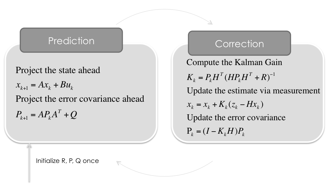
Multidimensional Kalman-Filter
Some Python Implementations of the Kalman Filter
####See Vimeo for some Explanations.
Kalman Filter with Constant Velocity Model
Situation covered: You drive with your car in a tunnel and the GPS signal is lost. Now the car has to determine, where it is in the tunnel. The only information it has, is the velocity in driving direction. The x and y component of the velocity (x˙ and y˙) can be calculated from the absolute velocity (revolutions of the wheels) and the heading of the vehicle (yaw rate sensor).
View IPython Notebook ~ See Vimeo
Kalman Filter with Constant Acceleration Model
in 2D
Situation covered: You have an acceleration sensor (in 2D: $\ddot x¨ and y¨) and try to calculate velocity (x˙ and y˙) as well as position (x and y) of a person holding a smartphone in his/her hand.
View IPython Notebook ~ See Vimeo
Second example is the same dynamic model but this time you measure the position as well as the acceleration. Both values have to be fused together with the Kalman Filter. Situation covered: You have an acceleration sensor (in 2D: x¨ and y¨) and a Position Sensor (e.g. GPS) and try to calculate velocity (x˙ and y˙) as well as position (x and y) of a person holding a smartphone in his/her hand.
View IPython Notebook ~ See Vimeo
in 3D
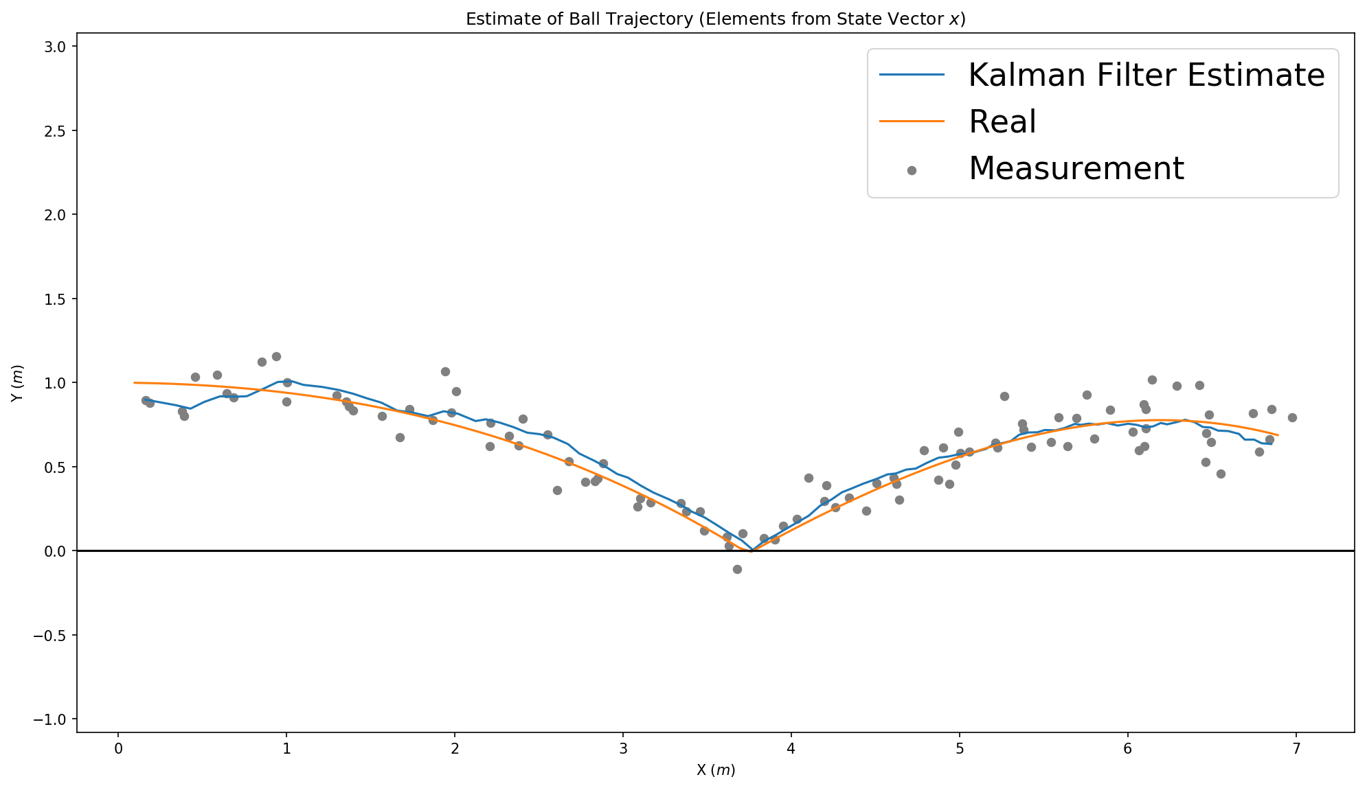
Third example is in 3D space, so the state vector is 9D. This model is for ball tracking or something else in 3D space.
Adaptive Kalman Filter with Constant Velocity Model
Here the Measurement Covariance Matrix R is calculated dynamically via the maximum likelihood of the acutal standard deviation of the last measurements.
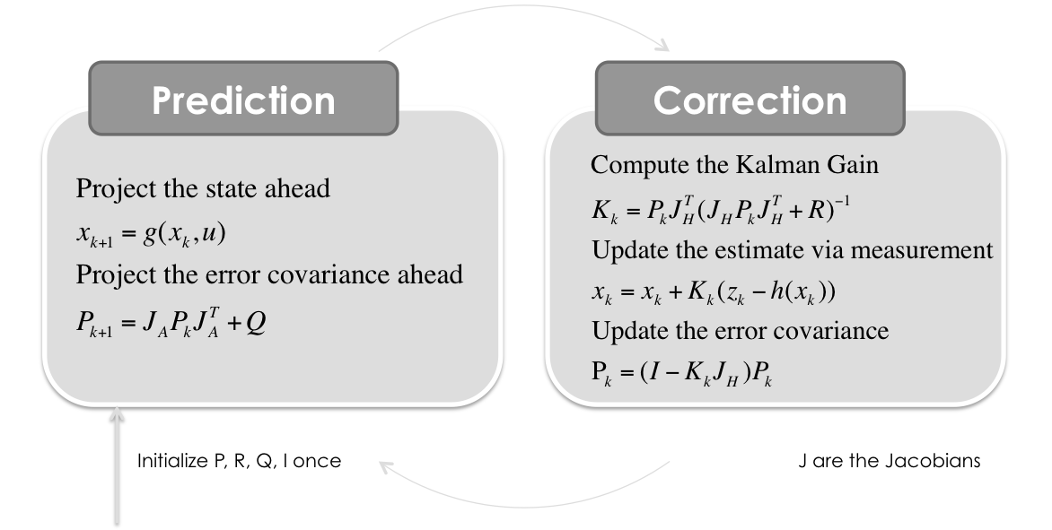
Extended Kalman Filter
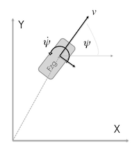
Extended Kalman Filter with Constant Turn Rate and Velocity (CTRV) Model
Situation covered: You have an velocity sensor which measures the vehicle speed (v) in heading direction (ψ) and a yaw rate sensor (ψ˙) which both have to fused with the position (x & y) from a GPS sensor.
View IPython Notebook ~ See Vimeo
License
CC-BY-SA2.0 Lizenz


