Information gain is calculated using a statistical measure called Entropy. Entropy is a widely used concept in the fields of Physics, Mathematics, Computer Science (information theory), and more. You may have come across the idea of entropy in thermodynamics, societal dynamics, and a number of other domains. In electronics and computer science, the idea of entropy is usually derived from Shannon's description of entropy to measure the information gain against some cost incurred in the process. In this lesson, we shall look at how this works with the simple example we introduced in the previous lesson.
You will be able to:
- Explain the process for selecting the best attribute for a split
- Calculate entropy and information gain by hand for a simple dataset
- Compare and contrast entropy and information gain
Entropy is a measure of disorder or uncertainty.
The measure is named after Claude Shannon, who is known as the "father of information theory". Information theory provides measures of uncertainty associated with random variables. These measures help calculate the average information content one is missing when one does not know the value of the random variable. This uncertainty is measured in bits, i.e., the amount of information (in bits) contained per average instance in a stream of instances.
Conceptually, information can be thought of as being stored or transmitted as variables that can take on different values. A variable can be thought of as a unit of storage that can take on, at different times, one of several different specified values, following some process for taking on those values. Informally, we get information from a variable by looking at its value, just as we get information from an email by reading its contents. In the case of the variable, the information is about the process behind the variable.
The entropy of a variable is the "amount of information" contained in the variable.
This amount is not only determined by the number of different values the variable can take, just as the information in an email is not quantified just by the number of words in the email or the different possible words in the language of the email. Informally, the amount of information in an email is proportional to the amount of “surprise” its reading causes.
For example, if an email is simply a repeat of an earlier email, then it is not informative at all. On the other hand, if, for example, the email reveals the outcome of an election, then it is highly informative. Similarly, the information in a variable is tied to the amount of surprise the value of that variable causes when revealed.
Shannon’s entropy quantifies the amount of information in a variable, thus providing the foundation for a theory around the notion of information.
In terms of data, we can informally describe entropy as an indicator of how messy your data is. A high degree of entropy always reflects "messed-up" data with low/no information content. The uncertainty about the content of the data, before viewing the data remains the same (or almost the same) as that before the data was available.
In a nutshell, higher entropy means less predictive power when it comes to doing data science with that data.
Decision trees aim to tidy the data by separating the samples and re-grouping them in the classes they belong to.
Because decision trees use a supervised learning approach, we know the target variable of our data. So, we maximize the purity of the classes as much as possible while making splits, aiming to have clarity in the leaf nodes. Remember, it may not be possible to remove the uncertainty totally, i.e., to fully clean up the data. Have a look at the image below:
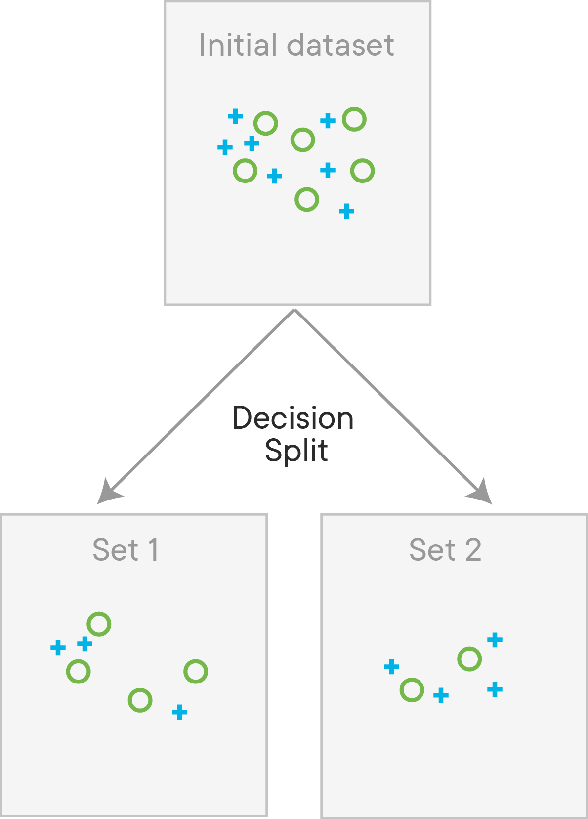
We can see that the split has not FULLY classified the data above, but the resulting data is tidier than it was before the split. By using a series of such splits that focus on different features, we try to clean up the data as much as possible in the leaf nodes. At each step, we want to decrease the entropy, so entropy is computed before and after the split. If it decreases, the split is retained and we can proceed to the next step, otherwise, we must try to split with another feature or stop this branch (or quit, in which case we claim that the current tree is the best solution).
Let's pretend we have a sample, True and False. Of the
Let's assume our boss brings us the dataset
If we know these ratios, we can calculate the entropy of the dataset
Don't worry too much about this equation yet -- we'll dig deeper into what it means in a minute.
The equation above tells us that a dataset is considered tidy if it only contains one class (i.e. no uncertainty or confusion). If the dataset contains a mix of classes for our target variable, the entropy increases. This is easier to understand when we visualize it. Consider the following graph of entropy in a dataset that has two classes for our target variable:
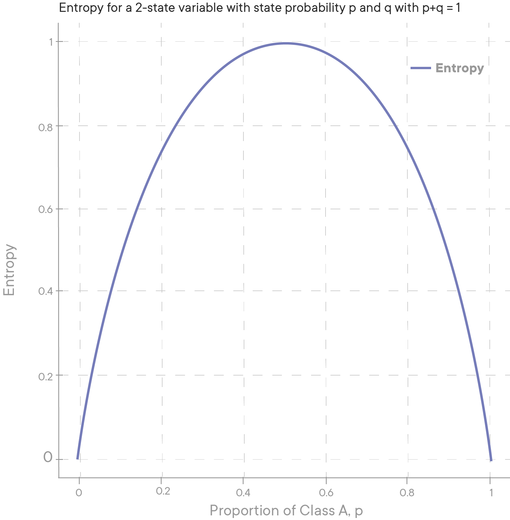
As you can see, when the classes are split equally,
This is where the logic behind decision trees comes in -- what if we could split the contents of our sock drawer into different subsets, which might divide the drawer into more organized subsets? For instance, let's assume that we've built a laundry robot that can separate items of clothing by color. If a majority of our socks are white, and a majority of our underwear is some other color, then we can safely assume that the two subsets will have a better separation between socks and underwear, even if the original chaotic drawer had a 50/50 mix of the two!
Now that we have a good real-world example to cling to, let's get back to thinking about the mathematical definition of entropy.
Entropy
We saw how to calculate entropy for a two-class variable before. However, in the real world we deal with multiclass problems very often, so it would be a good idea to see a general representation of the formula we saw before. The general representation is:
When
Information gain is an impurity/uncertainty based criterion that uses the entropy as the measure of impurity.
There are several different algorithms out there for creating decision trees. Of those, the ID3 algorithm is one of the most popular. Information gain is the key criterion that is used by the ID3 classification tree algorithm to construct a decision tree. The decision tree algorithm will always try to maximize information gain. The entropy of the dataset is calculated using each attribute, and the attribute showing highest information gain is used to create the split at each node. A simple understanding of information gain can be written as:
A weighted average based on the number of samples in each class is multiplied by the child's entropy, since most datasets have class imbalance. Thus the information gain calculation for each attribute is calculated and compared, and the attribute showing the highest information gain will be selected for the split. Below is a more generalized form of the equation:
When we measure information gain, we're really measuring the difference in entropy from before the split (an untidy sock drawer) to after the split (a group of white socks and underwear, and a group of non-white socks and underwear). Information gain allows us to put a number to exactly how much we've reduced our uncertainty after splitting a dataset
Where:
-
$H(S)$ is the entropy of set$S$ -
$t$ is a subset of the attributes contained in$A$ (we represent all subsets$t$ as$T$ ) -
$p(t)$ is the proportion of the number of elements in$t$ to the number of elements in$S$ -
$H(t)$ is the entropy of a given subset$t$
In the ID3 algorithm, we use entropy to calculate information gain, and then pick the attribute with the largest possible information gain to split our data on at each iteration.
So far, we've focused heavily on the math behind entropy and information gain. This usually makes the calculations look scarier than they actually are. To show that calculating entropy/information gain is actually pretty simple, let's take a look at an example problem -- predicting if we want to play tennis or not, based on the weather, temperature, humidity, and windiness of a given day!
Our dataset is as follows:
| outlook | temp | humidity | windy | play |
|---|---|---|---|---|
| overcast | cool | high | Y | yes |
| overcast | mild | normal | N | yes |
| sunny | cool | normal | N | yes |
| overcast | hot | high | Y | no |
| sunny | hot | normal | Y | yes |
| rain | mild | high | N | no |
| rain | cool | normal | N | no |
| sunny | mild | high | N | yes |
| sunny | cool | normal | Y | yes |
| sunny | mild | normal | Y | yes |
| overcast | cool | high | N | yes |
| rain | cool | high | Y | no |
| sunny | hot | normal | Y | no |
| sunny | mild | high | N | yes |
Let's apply the formulas we saw earlier to this problem:
Out of 14 instances, 9 are classified as yes, and 5 as no. So:
The current entropy of our dataset is 0.94. In the next lesson, we'll see how we can improve this by subsetting our dataset into different groups by calculating the entropy/information gain of each possible split, and then picking the one that performs best until we have a fully fleshed-out decision tree!
In this lesson, we looked at calculating entropy and information gain measures for building decision trees. We looked at a simple example and saw how to use these measures to select the best split at each node. Next, we calculate these measures in Python, before digging deeper into decision trees.