我们希望将《计算方法》课程中的理论内容通过Python语言进行实现,并将其运用到实际问题之中。 作为一个对计算机稍微有一定了解的学习者,深知将理论转化为实际往往是存在困难的。通常发展了一门新的理论,并将其转化为技术,这期间需要很长的时间来逐步完善并提高效率。
更重要的是,我们认为这门课程中的一些方法是形象生动而有趣的。可能在更高级的模块中集成了比这些先进得多的算法,但是这并不重要,我们希望用这本书中的方法来解决一些适合于我们的需求的问题。
This repository is used to create a project on lesson "Numerical Analysis" and practically use the method we have learned in problem solving. As a learner who knows only a little about computer and programming, I know that there must exist difficulties in the transformation from theory to practice. It takes long time when the theory generally improves efficiency as technical tools.
From our perspective, some methods in this lesson are really interesting and fantastic. Maybe some much advanced technique has been used in popular modules, however, it is not important while we hope that the method in our textbook can solve the problem we faced and adapted to our demand.
- 非线性方程数值解/Numerical Solution to Nonlinear Equation
- 线性方程组LU分解/System of Linear Equation——LU Decomposition
- 线性方程组迭代法/Recursive way to solve the System of Linear Equation
- 插值与拟合/Interpolation and Fitting
- 数值积分/Numerical Integral
- 插值型数值积分
- 牛顿科特斯公式/Newton-Cotes Method
- 复化求积公式/Composite Integral
- 常微分方程数值解/Numerical Solution in Ordinary Differential Equation
基本原理
在这个部分中我们将利用循环完成迭代的操作,需要手动输入迭代公式
,具体代码如下:
import numpy as np
import sympy as sp
g = lambda x: x**2-3*x**(1/2)+4 # Here input your recursive function
x0 = 1 # Your initial point
n = 10 # Your iteration times
residual = 0.001 # Your tolerance

def Recursive_Method(g,x0,n,residual):
    x = np.zeros(n+1)
    x[0] = x0
    for index in range(1,n+1):
        x[index] = g(x[index-1])
        difference = x[index] - x[index-1]
        if np.abs(x[index]-x[index-1])<residual:
            print("Iteration %r: x=%r, difference=%r <= Residual=%r" %(index,x[index],difference,residual))
            break
        else:
            print("Iteration %r: x=%r, difference=%r" %(index,x[index],difference))
    print("Terminal: The final result is %r" % x[index])
    return x[index]

Recursive_Method(g,x0,n,residual)例如我们要使用求解
在
上的根,迭代10次或两次误差小于
,则使用以下的代码
g = lambda x: 0.5*(10-x**3)**0.5
Recursive_Method(g,1.5,10,1e-5)
得到的结果为:
Iteration 1: x=1.2869537676233751, difference=-0.2130462323766249
Iteration 2: x=1.4025408035395783, difference=0.11558703591620323
Iteration 3: x=1.3454583740232942, difference=-0.057082429516284172
Iteration 4: x=1.3751702528160383, difference=0.029711878792744173
Iteration 5: x=1.3600941927617329, difference=-0.015076060054305396
Iteration 6: x=1.3678469675921328, difference=0.0077527748303998223
Iteration 7: x=1.3638870038840212, difference=-0.0039599637081115802
Iteration 8: x=1.3659167333900399, difference=0.0020297295060187626
Iteration 9: x=1.3648782171936771, difference=-0.0010385161963628597
Iteration 10: x=1.3654100611699569, difference=0.00053184397627981106
Terminal: The final result is 1.3654100611699569
注意
- 本部分尚未加入是否发散的判断,因此要根据迭代结果进行发散的判断
- 请自行计算迭代式
,在输入过程中注意指数与根号的输入规范
具有特殊迭代格式的迭代法,对于的求解,采用格式:
能保证更快的收敛速度。这里,我们为了得到更为精确的结果,避免数值微分带来的误差和符号计算可能碰到的不确定性,要求手动输入函数,并同理使用迭代法中的方法:
f = lambda x: x**2+3*x+1 # Your function f(x)
f1 = lambda x: 2*x+3 # First order deviation of f(x)
x0 = 1 # The initial point
n = 100 # Iteration time
residual = 1e-5 # Tolerance

def Newton_Recursive(f,f1,x0,n,residual):
    x = np.zeros(n+1)
    x[0] = x0
    for index in range(1,n+1):
        x[index] = x[index-1]-f(x[index-1])/f1(x[index-1])
        difference = x[index] - x[index-1]
        if np.abs(x[index]-x[index-1])<residual:
            print("Iteration %r: x=%r, difference=%r <= Residual=%r" %(index,x[index],difference,residual))
            break
        else:
            print("Iteration %r: x=%r, difference=%r" %(index,x[index],difference))
    print("Terminal: The final result is %r" % x[index])
    return x[index]

Newton_Recursive(f,f1,x0,n,residual)
作为对比,我们依旧解决迭代法中10次尚未达到精度的例子:
求解
在
上的根,迭代10次或两次误差小于
。 此时,在牛顿法中,
。对应代码为:
f = lambda x: x**3+4*x**2-10
f1 = lambda x: 3*x**2+8*x
Newton_Recursive(f,f1,1.5,10,1e-5)
仅通过三次迭代就得到收敛结果
Iteration 1: x=1.3733333333333333, difference=-0.12666666666666671
Iteration 2: x=1.3652620148746266, difference=-0.0080713184587066777
Iteration 3: x=1.3652300139161466, difference=-3.2000958479994068e-05
Iteration 4: x=1.3652300134140969, difference=-5.0204973511824846e-10 <= Residual=1e-05
Terminal: The final result is 1.3652300134140969
非线性方程组的求解是一个更加困难的问题,非线性方程组的解往往具有多个,也可能不存在,并且对初值十分敏感,我们在这里使用牛顿-拉夫逊法进行非线性方程组的迭代求解。这种方法是牛顿法的推广,但存在很多的局限性。
,其中
为Jacobi矩阵(全体一阶偏导矩阵)
从简化的角度,我们仅分析三个方程组三个未知数的情形,解决代码如下:
def Jacobi_Matrix(f1,f2,f3,ak,bk,ck):
    a = sp.Symbol('a')
    b = sp.Symbol('b')
    c = sp.Symbol('c')
    F = [f1,f2,f3]
    X = [a,b,c]
    n = len(F)
#    F_1 = np.array([[a,b,c],
#                    [a,b,c],
#                    [a,b,c]])
    F_1v = np.zeros((n,n))
    for i in range(n):
        for j in range(n):
#            F_1[i,j] = sp.diff(F[i],X[j])
            storage = sp.diff(F[i],X[j])
            F_1v[i,j] = storage.evalf(subs = {a:ak,b:bk,c:ck})
    #F1v = F_1.evalf(subs = {X:X0})
    return np.linalg.inv(F_1v)

def Newton_Recursive_Multi(f1,f2,f3,a0,b0,c0,n):
    a = sp.Symbol('a')
    b = sp.Symbol('b')
    c = sp.Symbol('c')
    x = np.zeros((3,n+1))
    x[0,0] = a0
    x[1,0] = b0
    x[2,0] = c0
    for k in range(n):
        if np.min(np.abs(x[:,k+1]-x[:,k]))>100:
            return "Error with divergence"
#            print("Error")
        else:
            if np.max(np.abs(x[:,k+1]-x[:,k]))>1e-5:
                F1 = f1.evalf(subs = {a:x[0,k],b:x[1,k],c:x[2,k]})
                F2 = f2.evalf(subs = {a:x[0,k],b:x[1,k],c:x[2,k]})
                F3 = f3.evalf(subs = {a:x[0,k],b:x[1,k],c:x[2,k]})
                F1 = float(F1)
                F2 = float(F2)
                F3 = float(F3)
                F = np.array([F1,F2,F3])
                x[:,k+1] = x[:,k]-Jacobi_Matrix(f1,f2,f3,x[0,k],x[1,k],x[2,k])@F
            else:
                return x[:,:k+1]
#                print("Error")
return x在这里我们默认两次迭代之间最小的变化的绝对值超过100为收敛条件(这可能不是一个好的判断方法),当两次迭代最大变化绝对值小于1e-5则认为迭代法收敛。一个例子如下:
# f = [f1,f2,f3,f4,f5]'=0
# a* = 1 b* = 3 c* = 2
a = sp.Symbol('a')
b = sp.Symbol('b')
c = sp.Symbol('c')
f1 = a**2 + b - 2*c
f2 = 3*a + 2**b -c**3 - 3
f3 = a + b + c - 6
a0 = 10
b0 = 25
c0 = 80
n = 100
solution = Newton_Recursive_Multi(f1,f2,f3,a0,b0,c0,n)我们得到在初值为时的迭代结果为
(尽管在我构造这个非线性方程组时设定的解是
,下面我们再使用另一组初值进行迭代:
# f = [f1,f2,f3,f4,f5]'=0
# a* = 1 b* = 3 c* = 2
a = sp.Symbol('a')
b = sp.Symbol('b')
c = sp.Symbol('c')
f1 = a**2 + b - 2*c
f2 = 3*a + 2**b -c**3 - 3
f3 = a + b + c - 6
a0 = 1
b0 = 2.5
c0 = 3.3
n = 100
solution = Newton_Recursive_Multi(f1,f2,f3,a0,b0,c0,n)
这种情况下我们得到了我们想要的收敛结果。
本部分求解的线性方程组为行列式不为0的实方阵,用数学符号来表示,为:
其中
我们考虑将系数矩阵分解为一个同维度的下三角矩阵
和一个同维度的上三角矩阵
的乘积,即
之所以这样做,是因为对于的求解是相对容易的,可以先通过求解
再来求解
。
首先我们先对系数矩阵A进行判断并返回维度供后续使用
import numpy as np

""" Input Example
A = np.array([[1,3,5,9],
              [2,5,2,5],
              [9,3,4,1],
              [1,10,0,19]]) # Here input your coefficient matrix
b = np.array([10,24,31,42]) # Here input the vector
"""

def check(A):
    row = A.shape[0]
    col = A.shape[1]
    if row!=col:
        print("Input error: A is not a square matrix")
        return 0
    else:
        if np.linalg.det(A)==0:
            print("The determination of A is equal to zero")
            return 0
        else:
            if row == 1:
                print("The dimension of matrix is 1")
                return 0
            else:
                return row
获得检验矩阵并获得维度信息后,再根据矩阵乘法定义进行LU分解:
def Decomposition(A):
    if check(A) == 0:
        print("Error")
    else:
        print("det(A)=%r"%np.linalg.det(A))
        dim = check(A)
        L = np.eye(dim)
        U = np.zeros_like(A)
        U[0,:]=A[0,:]
        L[1:,0]=A[1:,0]/U[0,0]
        for r in range(1,dim):
            for l in range(1,r):
                L[r,l]=1/U[l,l]*(A[r,l]-L[r,:l]@U[:l,l])
            for u in range(r,dim):
                U[r,u]=A[r,u]-L[r,:r]@U[:r,u]
    print("L=\n",L,"\n","U=\n",U)
    return L,U
例如我们对下方矩阵A进行分解:
A = np.array([[1,3,5],
              [2,5,2],
              [9,3,4]
              ])
Decomposition(A)
得到结果为
det(A)=-151.0
L=
 [[  1.   0.   0.]
 [  2.   1.   0.]
 [  9.  24.   1.]]
 U=
 [[  1   3   5]
 [  0  -1  -8]
 [  0   0 151]]
再分别求解:
def Solve(A,b):
   L,U = Decomposition(A)
   y = np.linalg.solve(L,b)
   x = np.linalg.solve(U,y)
   print("y=\n",y,"\n","x=\n",x)
return y,x目标依然是求解线性方程组
此处的迭代法类似于迭代法,但迭代对象换成了矩阵和向量,依旧选择合适的
使得
以上迭代**导出不同收敛速度的Jacobi迭代法和Gauss-Seidel迭代法。为了后面更好地描述,我们定义以下记号:
Jacobi迭代的格式为
其中,矩阵D, L, U的分解为:
import numpy as np
import sympy as sp

def Decomposition(A):
    dim = A.shape[0]
    D = np.zeros_like(A)
    L = np.zeros_like(A)
    U = np.zeros_like(A)
    for r in range(dim):
        D[r,r] = A[r,r]
        for c in range(dim):
            if c<r:
                L[r,c] = -A[r,c]
            if c>r:
                U[r,c] = -A[r,c]
    return D,L,U
利用上方分解结果进行Jacobi迭代:
def Jacobi(A,x0,b,n):
    D,L,U = Decomposition(A)
    D_1 = np.linalg.inv(D)
    print("Inverse of D=\n",D_1)
    g = lambda x: D_1@(L+U)@x + D_1@b
    x = np.zeros((A.shape[0],n+1))
    x[:,0] = x0
    for iteration in range(1,n+1):
        x[:,iteration] = g(x[:,iteration-1])
        print("Iteration %d:"%iteration,"x=",x[:,iteration])
    return x
我们用上述代码完成书本中的例题:
求解方程组:
,取初值为
,迭代次数为10。
A = np.array([[8,-3,2],
              [4,11,-1],
              [2,1,4]])
b = np.array([20,33,12])
x0 = np.array([0,0,0])
Jacobi(A,x0,b,10)
结果为:
Inverse of D=
 [[ 0.125       0.          0.        ]
 [ 0.          0.09090909  0.        ]
 [ 0.          0.          0.25      ]]
Iteration 1: x= [ 2.5  3.   3. ]
Iteration 2: x= [ 2.875       2.36363636  1.        ]
Iteration 3: x= [ 3.13636364  2.04545455  0.97159091]
Iteration 4: x= [ 3.02414773  1.94783058  0.92045455]
Iteration 5: x= [ 3.00032283  1.9839876   1.00096849]
Iteration 6: x= [ 2.99375323  1.99997065  1.00384168]
Iteration 7: x= [ 2.99902857  2.0026208   1.00313072]
Iteration 8: x= [ 3.00020012  2.00063786  0.99983051]
Iteration 9: x= [ 3.00028157  1.99991182  0.99974048]
Iteration 10: x= [ 3.00003181  1.99987402  0.99988126]
Gauss-Seidel迭代的格式为
类似地,我们用以下代码进行实现:
def GS(A,x0,b,n):
    D,L,U = Decomposition(A)
    D_L = D-L
    D_L_1 = np.linalg.inv(D_L)
    print("Inverse of D-L=\n",D_L_1)
    g = lambda x: D_L_1@U@x + D_L_1@b
    x = np.zeros((A.shape[0],n+1))
    x[:,0] = x0
    for iteration in range(1,n+1):
        x[:,iteration] = g(x[:,iteration-1])
        print("Iteration %d:"%iteration,"x=",x[:,iteration])
    return x
Gauss-Seidel与Jacobi迭代的区别在于,每次迭代的过程中就代入迭代值加速收敛,因此其收敛速度更快,对于上面方程组,Gauss-Seidel迭代法的10次迭代结果为:
Inverse of D-L=
 [[ 0.125       0.          0.        ]
 [-0.04545455  0.09090909  0.        ]
 [-0.05113636 -0.02272727  0.25      ]]
Iteration 1: x= [ 2.5         2.09090909  1.22727273]
Iteration 2: x= [ 2.97727273  2.02892562  1.00413223]
Iteration 3: x= [ 3.00981405  1.99680691  0.99589125]
Iteration 4: x= [ 2.99982978  1.99968838  1.00016302]
Iteration 5: x= [ 2.99984239  2.00007213  1.00006077]
Iteration 6: x= [ 3.00001186  2.00000121  0.99999377]
Iteration 7: x= [ 3.00000201  1.9999987   0.99999932]
Iteration 8: x= [ 2.99999968  2.00000005  1.00000014]
Iteration 9: x= [ 2.99999998  2.00000002  1.        ]
Iteration 10: x= [ 3.00000001  2.          1.        ]
多项式具有以下的形式
多项式插值的原理是带入数据从而解出多项式中的系数,简而言之,就是解一个线性方程组,方程数等于所给的数据对的数量,而多项式最高次数为方程数减1。出于简化的目的,我们不想在这里研究线性方程组解的个数究竟是无、唯一还是无穷,我们只考虑最简单的情况,即n对数据解n-1次多项式的情形。
import numpy as np
import sympy as sp
""" Data Input: We input data in an array which has the form of (x,y)

data = np.array([[1,-1],
                 [2,-1],
                 [3,1]
                 ])
"""
def Polynomial(data):
    dim = data.shape[0]
    A = np.zeros((dim,dim))
    for c in range(dim):
        g = lambda x:x**c
        A[:,c] = g(data[:,0])
    soln = np.linalg.solve(A,data[:,1])
    for index in range(dim):
        print("c%d = %r"%(index,soln[index]))
    return soln

def Polynomial_predict(data,x):
    coefficient = Polynomial(data)
    result = 0
    for index in range(len(coefficient)):
        g = lambda x: x**index
        result = result + g(x)*coefficient[index]
    return result
例如:
求解下方数据对应的插值多项式:
(x1,y1)=(1,0)
(x2,y2)=(2,4)
(x3,y3)=(3,8)
并预测在x=1.5时的值。
代码为:
data = np.array([[1,0],
                 [2,4],
                 [3,8]])
Polynomial(data)
Polynomial_predict(data,1.5)
结果:
array([-4.,  4., -0.])
2.0
即
拉格朗日插值公式原理如下:
其中
代码如下:
def li_calc(data,i):
    dim = data.shape[0]
    x = sp.Symbol('x')
    li = 1
    for index in range(dim):
        if index != i:
            li = li*(x-data[index,0])/(data[i,0]-data[index,0])
        else:
            li = li
    return li

def Lagrangian(data):
    dim = data.shape[0]
    L = 0
    for index in range(dim):
        L = L +li_calc(data,index)*data[index,1]
    return L.expand()

def Lagrangian_predict(data,y):
    result = Lagrangian(data)
    x = sp.Symbol('x')
    return result.evalf(subs = {x:y})
选取课本案例:
求解下方数据对应的拉格朗日Lagrangian插值多项式:
(x1,y1)=(1,-1)
(x2,y2)=(2,-1)
(x3,y3)=(3,1)
并预测在x=1.5时的值。 代码如下:
data = np.array([[1,-1],
                 [2,-1],
                 [3,1]])
Lagrangian(data)
Lagrangian_predict(data,1.5)
结果如下:
x**2 - 3*x + 1
-1.25000000000000
此处牛顿插值需要使用差商的概念。
绘制差商表:
def Divided_difference(data):
    dim = data.shape[0]
    D = np.zeros((dim,dim+1))
    D[:,0] = data[:,0]
    D[:,1] = data[:,1]
    diff = 1
    for column in range(2,dim+1):
        for row in range(diff,dim):
            D[row,column] = (D[row,column-1]-D[row-1,column-1])/(D[row,0]-D[row-diff,0])
        diff = diff+1
    return D
得出牛顿插值公式和拟合结果:
def Newton(data):
    Coefficient = Divided_difference(data)
    x = sp.Symbol('x')
    Newton = 0
    X = 1
    dim = data.shape[0]
    for index in range(dim):
        Newton = Newton + Coefficient[index,index+1]*X
        X = X*(x-Coefficient[index,0])
    return Newton.expand()
def Newton_predict(data,y):
    result = Newton(data)
    x = sp.Symbol('x')
    return result.evalf(subs = {x:y})
给定数据并求在x=1.5的拟合值:
(0,2), (1,-3), (2,-6), (3,11)。
运行代码:
data = np.array([[0,2],
                [1,-3],
                [2,-6],
                [3,11]])
Divided_difference(data)
Newton(data)
Newton_predict(data,1.5)
得到差商表(第一列为x,第二列为y,其后为一阶、二阶、三阶差商)和牛顿插值多项式:
array([[  0.,   2.,   0.,   0.,   0.],
       [  1.,  -3.,  -5.,   0.,   0.],
       [  2.,  -6.,  -3.,   1.,   0.],
       [  3.,  11.,  17.,  10.,   3.]])
3.0*x**3 - 8.0*x**2 + 2.0
-5.87500000000000
最小二乘拟合与插值不同。在插值点处,插值函数的值是精确的,但不能保证其他点的状况。而拟合则要求均方误差最小,在给定数据点的值并不一定准确。我们利用矩阵形式来推导,发现当均方误差最小时(一阶条件),可以解出。在非奇异条件下,可求解
。
为此,我们假设拟合函数为:
实现代码如下:
def LeastSquare(data,g1,g2,g3):
    dim = data.shape[0]
    A = np.zeros((dim,3))
    A[:,0] = g1(data[:,0])
    A[:,1] = g2(data[:,0])
    A[:,2] = g3(data[:,0])
    if np.linalg.det(A.T@A)!=0 :
        result = (np.linalg.inv(A.T@A))@(A.T)@(data[:,1])
        print("Coefficient: ",result)
        return result
    else:
        print("The inverse of A'A doesn't exist")
return 0该部分的代码存在偷懒的部分,我们为了简单,只选取了三个可能的函数。假设我们要利用数据点和函数
完成最小二乘拟合,则需要:
data = np.array([[1,-3],
                [2,-6],
                [3,11],
                [4,7],
                [5,14]])
g1 = lambda x: np.exp(x)
g2 = lambda x: x
g3 = lambda x: 1/x
LeastSquare(data,g1,g2,g3)
得到结果为:
Coefficient: [ 0.02822754 2.23012035 -7.19255383]
即拟合结果为
如果我们希望知道插值与拟合的效果如何,一个最简单的方法就是通过图像进行分析。尽管课本中并不要求我们绘图,但是我们在这里尝试实现这一点,因为这样很Coooooool!
def plot(data):
    xmin = np.min(data[:,0])
    xmax = np.max(data[:,0])
    ymin = np.min(data[:,1])
    ymax = np.max(data[:,1])
    x0 = np.linspace(xmin-0.5,xmax+0.5,100)
    x = sp.Symbol('x')
    fig, ax = plt.subplots(dpi=120)
    ax.set_xlim(xmin-1,xmax+1)
    ax.set_ylim(ymin-1,ymax+1)
    ax.scatter(data[:,0],data[:,1],marker='v')
    Poly = Polynomial_predict(data,x0)
    Lagr = Lagrangian(data)
    Newt = Newton(data)
    L = np.zeros(100)
    N = np.zeros(100)
    index = 0
    for tick in x0:
        L[index] = Lagr.evalf(subs = {x:tick})
        N[index] = Newt.evalf(subs = {x:tick})
        index = index+1
    ax.plot(x0,Poly,'r-',label='Ploynomial',alpha=0.3)
    ax.plot(x0,L,'b-',label='Lagrangian',alpha=0.3)
    ax.plot(x0,N,'g-',label='Newton',alpha=0.3)
    ax.legend()
    ax.set_title("Plot")
    fig.show()
plot(data)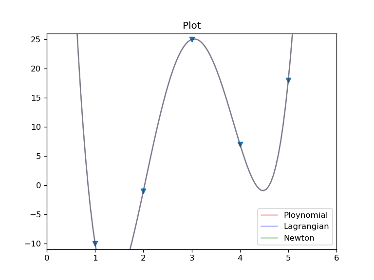
利用插值函数对被积函数
进行估计,再利用插值函数的优良积分性质求解积分
我们依次将带入,当存在某个正整数
成立但对于
不成立时,则称数值积分代数精度为
阶
牛顿-科特斯公式相比于一般插值型积分,其特点在于将积分区间等距分割,对于区间的等距分割,我们只需要利用步长
和分割段数
即可刻画整个数值积分。
当区间被分割为1份(即不分割)时,牛顿-柯特斯公式退化成梯形公式:
def trapezium(data,a,b):
    " Integral from ath data to bth data "
    #dim = b-a
    x = data[a-1,0]
    y = data[b-1,0]
    fx = data[a-1,1]
    fy = data[b-1,1]
return (y-x)/2*(fx+fy)当区间被分割为2份(即不分割)时,牛顿-柯特斯公式退化成Sinpson公式:
def sinpson(data,a,b):
    " Integral from ath data to bth data "
    dim = b-a
    if dim%2 != 0:
        return "Error"
    else:
        x = data[a-1,0]
        #xy = data[(b+a)/2-1,0]
        y = data[b-1,0]
        fx = data[a-1,0]
        fy = data[b-1,0]
        fxy = data[(b+a)/2-1,0]
return (y-x)/6*(fx+4*fxy+fy)在每个小区间上使用梯形公式再加总
def com_trapezium(data):
    dim = data.shape[0]
    a = data[0,0]
    b = data[dim-1,0]
    h = (b-a)/(dim-1)
    result = data[0,1]+data[dim-1,1]
    for index in range(1,dim-1):
        result = result + 2*data[index,1]
return result*h/2在每个小区间上使用复化Sinpson公式再加总
def com_sinpson(data):
    dim = data.shape[0]
    a = data[0,0]
    b = data[dim-1,0]
    h = (b-a)/(dim-1)*2
    result = data[0,1]+data[dim-1,1]
    #times = (dim-1)/2
    for index in range(1,dim-1):
        if index%2 != 0:
            result = result + 4*data[index,1]
        else:
            result = result + 2*data[index,1]
    return result*h/6
例如我们要求解以下问题
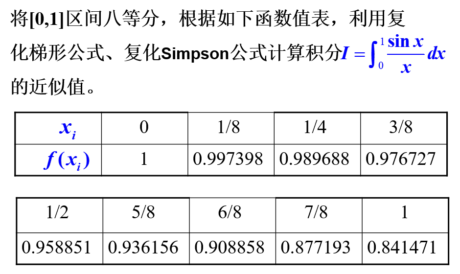
使用如下代码求解:
data = np.array([[0,1],
                 [0.125,0.997398],
                 [0.25,0.989688],
                 [0.375,0.976727],
                 [0.5,0.958851],
                 [0.625,0.936156],
                 [0.75,0.908858],
                 [0.875,0.877193],
                 [1,0.841471]])
com_trapezium(data)
com_sinpson(data)
运行结果为
0.94570081249999993
0.94609004166666677
在此仅考虑常微分方程初值问题

Euler法使用折现逼近曲线,通过初值条件逐次迭代得出整条曲线
import numpy as np
import matplotlib.pyplot as plt

""" Input:
Interval: [a,b]
Step: h
Differential: f(x,y)
Initial point: y(a) = y0
"""

def EulerMethod(a,b,h,f,y0):
    if b>a:
        step = int((b-a)/h+1)
        x = np.linspace(a,b,step)
        y = np.zeros_like(x)
        y[0]=y0
        for index in range(1,step):
            y[index] = y[index-1] + h*f(x[index-1],y[index-1])
        return y
    else:
return "Error"改进的Euler法在迭代过程中加入Euler法的估计值,使得迭代更加精确
def I_EulerMethod(a,b,h,f,y0):
if b>a:
step = int((b-a)/h+1)
x = np.linspace(a,b,step)
y = np.zeros_like(x)
ye = np.zeros_like(x)
y[0] = y0
ye[0] = y0
for index in range(1,step):
ye[index] = ye[index-1] + h*f(x[index-1],ye[index-1])
y[index] = y[index-1] + 0.5*h*(f(x[index-1],y[index-1])+f(x[index],ye[index]))
return y
else:
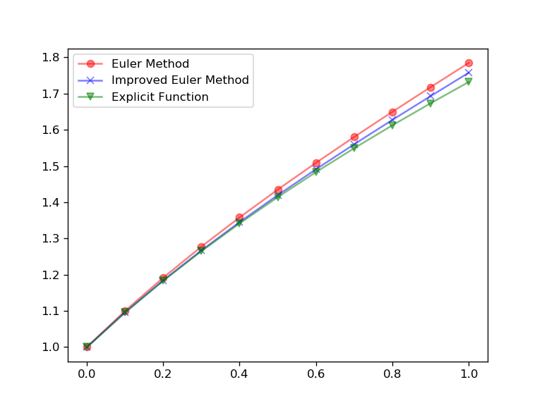
return "Error"此外,当我们知道解析解时,我们可以利用绘图得方法观察误差。为了实现这个很酷的功能,我们定义下方函数:
def Draw(a,b,h,f,y0,ft):
    step = int((b-a)/h+1)
    x = np.linspace(a,b,step)
    fig, ax = plt.subplots(dpi=120)
    ye = EulerMethod(a,b,h,f,y0)
    yie = I_EulerMethod(a,b,h,f,y0)
    yt = ft(x)
    ax.plot(x,ye,marker='o',color='r',alpha=0.5,label='Euler Method')
    ax.plot(x,yie,marker='x',color='b',alpha=0.5,label='Improved Euler Method')
    ax.plot(x,yt,marker='v',color='g',alpha=0.5,label='Explicit Function')
    ax.legend()
    fig.show()
    return 0
作为例子,我们尝试求解以下的例子
a = 0
b = 1
h = 0.1
f = lambda x,y: y-2*x/y
y0 = 1
ft = lambda x: np.sqrt(1+2*x)

EulerMethod(a,b,h,f,y0)
I_EulerMethod(a,b,h,f,y0)
Draw(a,b,h,f,y0,ft)
求得结果为
array([ 1.        ,  1.1       ,  1.19181818,  1.27743783,  1.3582126 ,
        1.43513292,  1.50896625,  1.58033824,  1.64978343,  1.71777935,
        1.78477083])
array([ 1.        ,  1.09590909,  1.18438953,  1.26711005,  1.34524979,
        1.41969469,  1.49114658,  1.56018901,  1.62733006,  1.69303203,
        1.7577335 ])