BorderRegion_KDE is a program to calculate a geographical Kernel Density Estimation (KDE) polygons derived from human mobility across country borders to map functional cross-border regions (e.g. Aagesen et al. 2023). This program helps to reveal functioning border regions, and transnational spaces in general, from the perspective of people as KDE indicates the probability density estimation for cross-border mobility from both side of the border.
This program imports unique cross-border movement vectors, processes movement vector data to calculate KDE levels, and geographically visualize KDEs in case of European countries. Yet, the program is generic and can be used globally once input data is updated, accordingly. The program has various parameter options for calculating KDEs, see the Usage section for further details.
In addition, BorderRegion_KDE program has few pre-processing features such as 1) converting H3 coordinates to Lat and Lon coordinates and 2) calculating the distance between start (origin) and end (destination) point of a mobility vector for defining what mobility vectors by distance are included for KDE calculation.
The work is conducted as a part of the BORDERSPACE – Tracing Interactions and Mobilities Beyond State Borders: Towards New Transnational Spaces project at the Digital Geography Lab, University of Helsinki.
This program has dummy data which you can try to see if it works as it should on your computer. Before you can run the program, a .env file has to be created (instructions below) from where the get_dotenv file retrieves the paths and filenames for the program. Other than that, everything else is set up for you to test the program with the dummy data. The dummy data works currently only for the KDE plot and not for the H3 to geo conversion. The distance is also already calculated in the dummy data, so no need to calculate the distance between points. To test the program with the dummy data, follow the installation steps below and create a .env file, everything else should have been already taken care of.
1. Navigate to a proper directory in your command line.
2. Clone the GitHub repository with the command below:
git clone https://github.com/DigitalGeographyLab/BorderRegion_KDE.git
3. Install Poetry if you don't have it installed already. More about installing Poetry here
4. Navigate into the BorderRegion_KDE folder.
5. Use Poetry to install all project dependencies with the command below, make sure you're inside the git repository in your command line:
poetry install
6. Use Poetry to active the virtual environment with this command:
poetry shell
7. After everything is installed and set upped, navigate to the src file and create a .env file in the root directory and follow the preparations (Instructions below)
This section gives an overview of the program and gives guidance on where and how the user should start the program as well as an illustration of the program structure.
- In the root directory, a .env file has to be created. In the .env file, the paths and filenames are defined so that the program finds the files. When using the dummy data, the user can copy and paste the text below into the .env file:
DATA_FOLDER_PATH = './DummyData/'
OUTPUT_FOLDER_PATH = './OutputFolder/'
OUTPUT_ALL = 'output_all/'
FILE_NAME_FOR_KDE_ANALYIS = 'pt_es_dummy_data_with_Haversine_distance.csv'
FILE_NAME_FOR_GPKG = 'pt_es_dummy_data_borders.gpkg'
- In the root directory, a .env file has to be created. When the user is using their own data or file structure, they need to add those paths and filenames to the .env file.
- Within the CountryCodes folder there is the lst_of_cntr_od file which contains a list of country pairs, change the content of this list if your country pairs are some others.
- The program's default EPSG is 3035 (ETRS89-extended / LAEA Europe). To change the EPSG, navigate to the kde_handler file in the KDE folder, and change the program_epsg parameter to your desired EPSG.
- Below you can find what data is needed for the program when using your own data:
If you have data with H3 coordinates, then a table with at least these columns is needed (start from step 1.)
- In the Preprocess folder, in the read_in_data_for_preprocess.py file, you can set/change the columns to load:
| CNTR_ID_start | CNTR_ID_end | h3_grid_res10_start | h3_grid_res10_end |
|---|---|---|---|
| ES | PT | 8e28e63c25bffff | 8e28e63c25bffff |
If you have data with lat and long coordinates, then a table with at least these columns is needed (start from step 2.):
| CNTR_ID_start | CNTR_ID_end | start_lat | start_lon | end_lat | end_lon |
|---|---|---|---|---|---|
| ES | PT | 42.34365181918523 | -3.6945932531644554 | 41.58460453590884 | -8.26853866397181 |
A geopackage (.gpkg) file with these columns for each country's polygons:
| NAME | CNTR_OD | geometry |
|---|---|---|
| Spain | ES | MULTIPOLYGON(((... |
| Portugal | PT | MULTIPOLYGON(((... |
N.B when using dummy data, jump straight to step 4 as the above steps are already done to the dummy data.
1. If the user's input data consists of H3 coordinates, then the user should first Preprocess the data so that those coordinates are converted to lat and long coordinates. The converted coordinates and the previous columns are saved to a DataFrame which is saved to a .csv file. N.B The program accepts input data that is either in .parquet or .csv file format.
2. After the user has converted the H3 coordinates or if the user already has a dataset with lat and long coordinates, then the user can calculate the distance (geodesic, haversine, great circle) between the starting and ending point on each row in the dataset, this will create a new column in the DataFrame which also is saved to a new .csv file. N.B .csv file format is the only format that the program accepts when loading data for the distance calculation.
3. When the user has done preprocessing (if that was needed), then the user does not have to redo the Preprocessing again as long as the created .csv files are saved and the paths to them are found in the .env file as these files will be used in the KDE visualization.
4. Now the user can proceed to the KDE visualization by selecting KDE in the first input question, this will print additional input questions about the KDE (questions below and example inputs):
-
Do you want to do a KDE for a specific country pair or all country pairs (pair/all): pair
-
What Bandwidth (i.e. search radius) in meters do you want to use (40km as 40000): 20000
-
Which kernel function do you want to use (gaussian/epanechnikov): epanechnikov
-
Which metric type do you want to use (euclidean/haversine): haversine
-
Do you want to limit movement distances (yes/no): yes
-
What is the maximum distance in kilometres you want to limit movement vectors (200km as 200): 300
-
Add first country abbreviation: ES
-
Add second country abbreviation: PT
5. The values in the parentheses, are examples or options of what the input can be. The slash(/) between the values indicates on an option between those two values and as indicates that any value is accepted but it has to be written like that so e.g if the user wants a bandwidth (search radius) of 20km, then it has to be written in meters as 20000.
6. After the input questions are answered, the program starts and shows plots, the first two plots are each country's own KDE plot and the third one is a combined KDE.
The following files are saved in the output folder:
- Combined KDE in .png format
- Combined KDE in .gpkg format
- Each country's KDE in .gpkg format (this is used by the program)
N.B Choosing haversine as the metric type can result in the below errors in some cases while euclidean always works.
    raise TypeError("`keep_geom_type` does not support {}.".format(geom_type))
TypeError: `keep_geom_type` does not support None.
In the StandaloneKDE folder is a class that is run independently and is not part of the bigger program, but uses the output from the program to visualize a combined KDE map.
- The merged_map_of_all_kdes.py consists of a stand-alone class that creates a merged map of all country pair KDEs, it is run from the src folder by:
python -m StandaloneKDE.merged_map_of_all_kdes
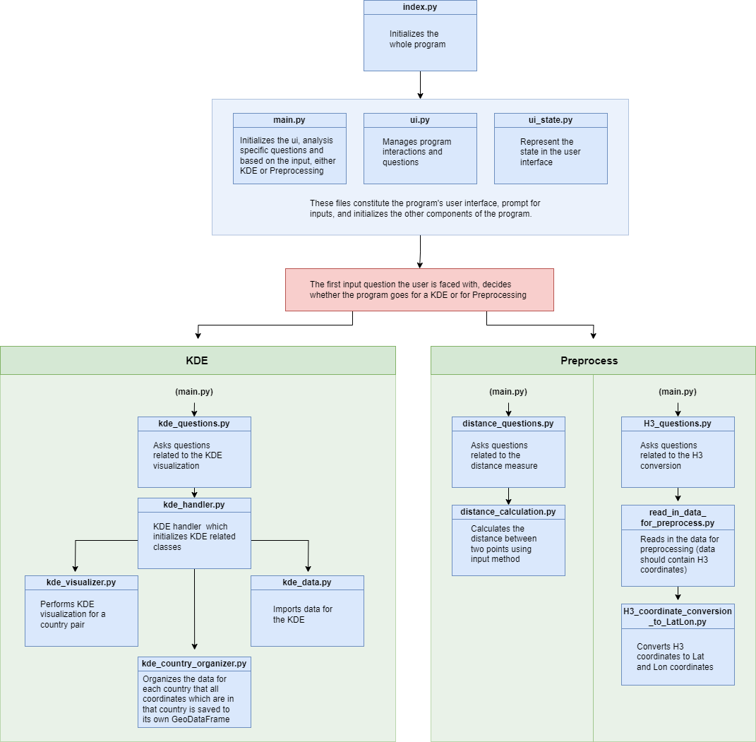
Below is an illustration of how the src folder is organized and a short description of what each class does for clarity. The blue boxes indicate a class (Python file) and the green boxes indicate a folder. All folders and files are not in this illustration as they function as support code for these classes.
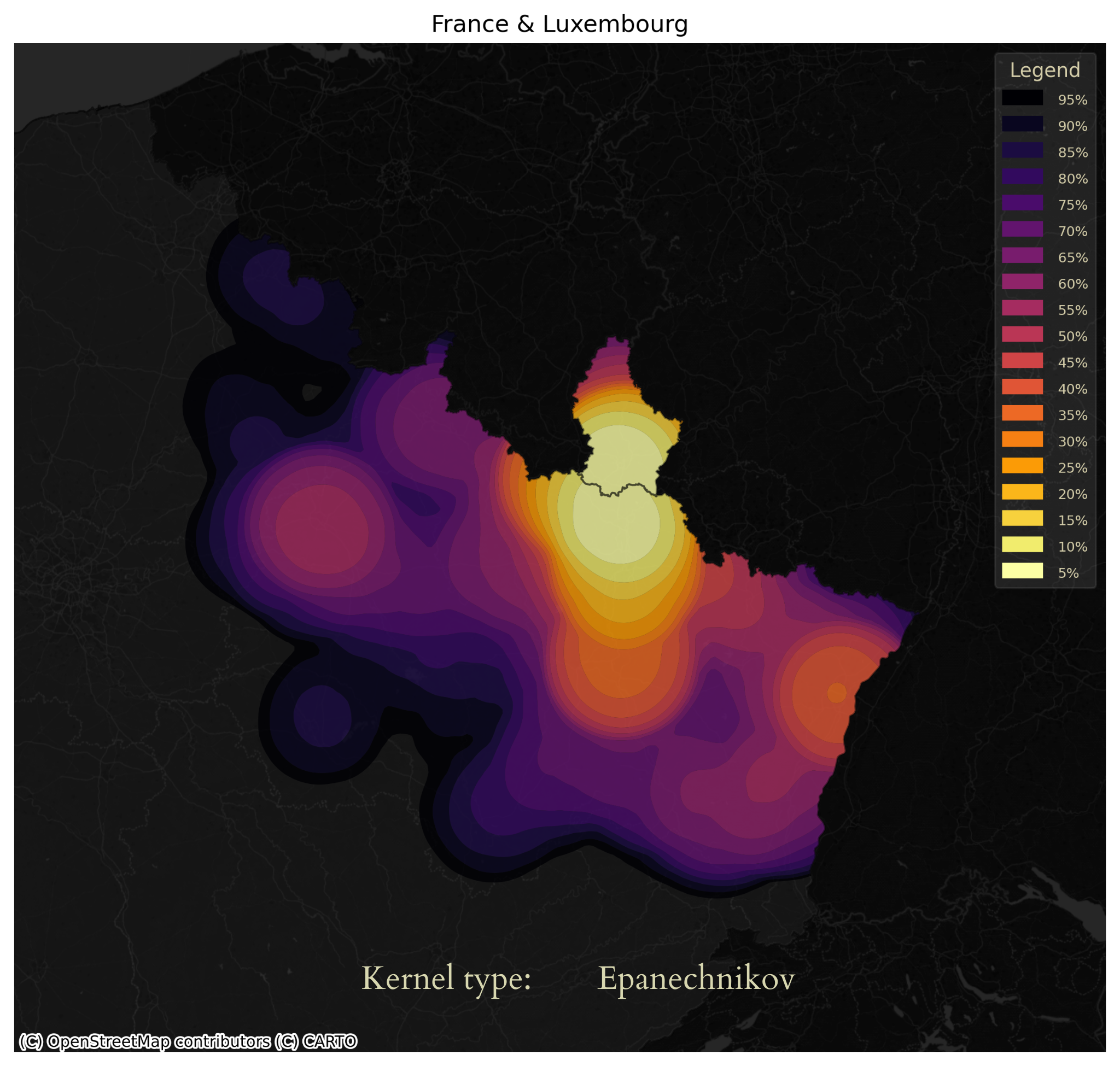
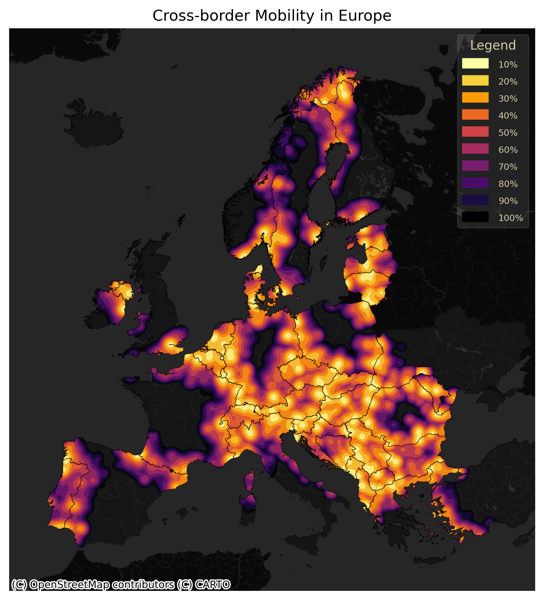
The output examples of the BorderRegion_KDE program are seen below (for more detailed examples see our Story Map). Here, the first example (map on the left) shows how a functional cross border region from cross-border human mobility between the two neighbouring countries, such as France and Luxembourg, is captured which is the default output of the program. Next, once several functional cross border regions between different country pairs are calculated, the program enables to further combine them together using the MergedMapOfAllKDEs class in the StandaloneKDE folder. As an example (map on the right), we combined all functional cross border region in Europe. For these examples, we used cross-border mobility derived from geolocated Twitter data (see, e.g. Järv et al. 2023; Aagesen et al. 2023).
 |
 |
|---|
If you use this program in your research or project, or develop it further, please refer back to us, as follows:
Söderholm, M., Aagesen, H., Väisänen, T., & Järv, O. (2023) BorderRegion_KDE. DOI: 10.5281/zenodo.10418690
Also in BibTeX:
@misc{Soderholm2023,
  title = {BorderRegion_KDE},
  shorttitle = {{{DigitalGeographyLab}}/BorderRegion_KDEr},
  author = {S{\"o}derholm, Michaela and Aagesen, H{\aa}vard and V{\"a}is{\"a}nen, Tuomas and J{\"a}rv, Olle},
  year = {2023},
  doi = {10.5281/zenodo.10418690},
  copyright = {GPLv3},
  howpublished = {Zenodo}
}
This work was supported by the Academy of Finland under Grant 331549 as a part of the BORDERSPACE project.
We also want to thank Martin Fleischmann for helping us to solve how to calculate geographically correct KDEs (see Disclaimer).
Our application relies on how KDE is implemented in sklearn Python library, instead of how it is done in seaborn. When writing this application, we found that seaborn's implementation of a two-dimensional KDE gets distorted or skewed when using geographical coordinates. We raised this issue with the developers, and found out this behaviour stems from scipy as it normalizes values for both X and Y axis. This approach assumes that X and Y represent completely different variables with entirely detached scales (e.g. GDP of a country and average life expectancy), which is a valid assumption for many cases. However, when working with geographical coordinates this assumption is wrong and will lead to erroneous results. We thank Martin Fleischmann for helping us troubleshoot the issue and contributing to the discussion with Seaborn developers.

