Clonotype Neighbor Graph Analysis (CoNGA) -- version 0.1.1

This repository contains the conga python package and associated scripts and workflows. conga was developed to detect correlation between T cell gene expression profile and TCR sequence in single-cell datasets. We've just recently added support for gamma delta TCRs and for B cells, too. conga is in active development right now so the interface may change in the next few months. Questions and requests can be directed to pbradley at fredhutch dot org or stefan.schattgen at stjude dot org.

Further details on conga can be found in the Nature Biotechnology manuscript "Integrating T cell receptor sequences and transcriptional profiles by clonotype neighbor graph analysis (CoNGA)" by Stefan A. Schattgen, Kate Guion, Jeremy Chase Crawford, Aisha Souquette, Alvaro Martinez Barrio, Michael J.T. Stubbington, Paul G. Thomas, and Philip Bradley, accessible here: https://www.nature.com/articles/s41587-021-00989-2 (original BioRxiv preprint here).

Running

Running conga on a single-cell dataset is a two- (or more) step process, as outlined below. Python scripts are provided in the scripts/ directory but analysis steps can also be accessed interactively in jupyter notebooks (for example, a simple pipeline and Seurat to conga in the top directory of this repo) or in your own python scripts through the interface in the conga python package. There's also a google colab notebook which you can and run. If you want to experiment before installing CoNGA locally you can save a copy of that notebook to your google drive, edit and run the pipeline, either on the provided examples or on data that you upload to the colab instance. The examples in the examples/ folder described below and in the jupyter notebooks feature publicly available data from 10x Genomics, which can be downloaded in a single zip file or at the 10x genomics datasets webpage.

SETUP: The TCR data is converted to a form that can be read by conga and then a matrix of TCRdist distances is computed. KernelPCA is applied to this distance matrix to generate a PC matrix that can be used in clustering and dimensionality reduction. This is accomplished with the python script scripts/setup_10x_for_conga.py for 10x datasets. For example:

python conga/scripts/setup_10x_for_conga.py --filtered_contig_annotations_csvfile vdj_v1_hs_pbmc3_t_filtered_contig_annotations.csv --organism human

ANALYZE: The scripts/run_conga.py script has an implementation of the main pipeline and can be run as follows:

python conga/scripts/run_conga.py --graph_vs_graph --gex_data data/vdj_v1_hs_pbmc3_5gex_filtered_gene_bc_matrices_h5.h5 --gex_data_type 10x_h5 --clones_file vdj_v1_hs_pbmc3_t_filtered_contig_annotations_tcrdist_clones.tsv --organism human --outfile_prefix tmp_hs_pbmc3

RE-ANALYZE: Step 2 will generate a processed .h5ad file that contains all the gene expression and TCR sequence information along with the results of clustering and dimensionality reduction. It can then be much faster to perform subsequent re-analysis or downstream analysis by "restarting" from those files. Here we are using the --all command line flag which requests all the major analysis modes:

python conga/scripts/run_conga.py --restart tmp_hs_pbmc3_final.h5ad --all --outfile_prefix tmp_hs_pbmc3_restart

See the examples section below for more details.

Installation

We highly recommend installing CoNGA in a virtual environment, for example using the anaconda package manager. Linux folks can check out the Dockerfile for a minimal set of installation commands. At the top of the google colab jupyter notebook (link to the notebook on colab) are the necessary installation commands from within a notebook environment.

Overview

Install the wonderful scanpy python package for single-cell analysis (docs). For example, with pip:

pip3 install scanpy[leiden]

Download the CoNGA github repository and (optional but recommended) compile the C++ TCRdist implementation; for example with git and make:

git clone https://github.com/phbradley/conga.git && cd conga/tcrdist_cpp && make

Make sure you have a tool that can convert .svg files to .png files, like inkscape, imagemagick convert, rsvg-convert, cairosvg (see below for details if you don't already have one).

NOTE we recognize that this is really lame, but right now you can't do import conga within a python script or notebook without first adding the install location to your python path (e.g., sys.path.append('/path/to/github-repos/conga/'). Running the scripts in the conga/scripts/ folder from the command line does not require this. We hope to smooth this out in the near future.

UPDATE Thanks to Neal Smith for helping us get set up with a very simple setup.py script, so now (in theory) one can cd to the top-most conga directory and type (after activating the relevant virtual environment):

pip install -e .

This should install the python dependencies and make it so you can just import conga without fiddling with sys.path. You will still need to have an svg--->png conversion tool like convert or inkscape installed (more details on that below).

Details

Here are some commands that would create an anaconda python environment for running CoNGA:

conda create -n conga_new_env ipython python=3.6
conda activate conga_new_env   # or: "source activate conga_new_env" depending on your conda setup
conda install seaborn scikit-learn statsmodels numba pytables
conda install -c conda-forge python-igraph leidenalg louvain notebook
conda install -c intel tbb # optional
pip install scanpy
pip install fastcluster # optional
conda install pyyaml #optional for using yaml-formatted configuration files for scripts

If you do not have the command line tool convert from Imagemagick, or Inkscape, installed, you could also add conda install -c conda-forge imagemagick. See the section below on SVG to PNG conversion for more details.

Next, clone the conga repository (type this command wherever you want the conga/ directory to appear):

git clone https://github.com/phbradley/conga.git

If you don't have git installed you could go click on the big green Code button on the CoNGA github page and download and unpack the software that way.

NEW We recently added a C++ implementation of TCRdist to speed neighbor calculations on large datasets and to compute the background TCRdist distributions for the new 'TCR clumping' analysis. This is not required by the core functionality described in the original manuscript, but we highly recommend that you compile the C++ TCRdist code using your C++ compiler.

We've successfullly used g++ from the GNU Compiler Collection (https://gcc.gnu.org/) to compile on Linux and MacOS, and from MinGw (http://www.mingw.org/) for Windows.

Using make on Linux or MacOS. (You can edit conga/tcrdist_cpp/Makefile to point to a C++ compiler other than g++)

cd conga/tcrdist_cpp
make

Or without make (for Windows)

cd conga/tcrdist_cpp
g++ -O3 -std=c++11 -Wall -I ./include/ -o ./bin/find_neighbors ./src/find_neighbors.cc
g++ -O3 -std=c++11 -Wall -I ./include/ -o ./bin/calc_distributions ./src/calc_distributions.cc
g++ -O3 -std=c++11 -Wall -I ./include/ -o ./bin/find_paired_matches ./src/find_paired_matches.cc

Even more details

The calculations in the conga manuscript were conducted with the following package versions:

scanpy==1.4.3 anndata==0.6.18 umap-learn==0.3.9 numpy==1.16.2 scipy==1.2.1 pandas==0.24.1 scikit-learn==0.20.2 statsmodels==0.9.0 python-igraph==0.7.1 louvain==0.6.1

which might possibly be installed with the following conda command:

conda create -n conga_classic_env ipython python=3.6 scanpy=1.4.3 umap-learn=0.3.9 louvain=0.6.1

Migrating Seurat data to CoNGA

We recommend using the write10XCounts function from the DropletUtils package for converting Seurat objects into 10x format for importing into CoNGA/scanpy.

require(Seurat)
require(DropletUtils)
hs1 <- readRDS('~/vdj_v1_hs_V1_sc_5gex.rds')

If the object contains only gene expression:

write10xCounts(x = hs1@assays$RNA@counts, path = './hs1_mtx/')
# import the hs1_mtx directory into CoNGA using the '10x_mtx' option

If the object contains both gene expression and antibody labeling:

# Concatenate the GEX and antibody labeling count matrices
# Here, ADT is the antibody labeling assay slot.

count_matrix <- rbind(hs1@assays$RNA@counts, hs1@assays$ADT@counts)

# create vector of feature type labels
features <- c(
  rep("Gene Expression", nrow(hs1@assays$RNA@counts)), 
  rep("Antibody Capture", nrow(hs1@assays$ADT@counts))
  )
              
# write out              
write10xCounts( count_matrix, 
                path = './hs1_mtx/',
                gene.id = rownames(count_matrix),
                gene.symbol = rownames(count_matrix),
                barcodes = colnames(count_matrix),
                gene.type = features,
                version = "3")
# import the hs1_mtx directory into CoNGA using the '10x_mtx' option

Merging multiple datasets into a single object for CoNGA analysis

This can be done in two easy steps using the setup_10x_clones.py and merge_samples.py scripts in conga.

SETUP: The TCR data for each sample being merge must be converted to a form that can be read by conga. This can be done using the python script scripts/setup_10x_for_conga.py for 10x datasets. By default the matrix of TCRdist distances calculated and reduced in dimensionality by KernelPCA, however, since these will need to be recalculated after merging we can skip this step with the --no_kpca flag.

python ~/conga/scripts/setup_10x_for_conga.py \
--filtered_contig_annotations_csvfile vdj_v1_hs_pbmc3_t_filtered_contig_annotations.csv \
--output_clones_file vdj_v1_hs_pbmc3_clones.tsv \
--organism human \
--no_kpca 

python ~/conga/scripts/setup_10x_for_conga.py \
--filtered_contig_annotations_csvfile sc5p_v2_hs_PBMC_10k_t_filtered_contig_annotations.csv \
--output_clones_file sc5p_v2_hs_PBMC_10k_clones.tsv \
--organism human \
--no_kpca

MERGE SAMPLES: The scripts/merge_samples.py script uses a tab-delimted file with three columns: "clones_file", "gex_data", "gex_data_type" specifying the paths to the clones file from step 1, it’s companion gex data, and the gex data type (e.g 10x_h5) for each sample:

clones_file	gex_data	gex_data_type
vdj_v1_hs_pbmc3_clones.tsv	vdj_v1_hs_pbmc_5gex_filtered_gene_bc_matrices_h5.h5	10x_h5
sc5p_v2_hs_PBMC_10k_clones.tsv	sc5p_v2_hs_PBMC_10k_filtered_feature_bc_matrix.h5	10x_h5

python ~/conga/scripts/merge_samples.py \
--samples pbmc_samples.txt \
--output_clones_file merged_pbmc_clones.tsv \
--output_gex_data merged_pbmc_gex.h5ad \
--organism human

The TCRdist distances are calculated and KernelPCA is applied to the matrix here.

ANALYZE: The merged AnnData object containing the gene expression and the merged clones file can now be analyzed using the scripts/run_conga.py script:

python ~/conga/scripts/run_conga.py \
--gex_data merged_pbmc_gex.h5ad \
--gex_data_type h5ad \
--clones_file merged_pbmc_clones.tsv \
--organism human \
--graph_vs_graph \
--outfile_prefix ../merged_pbmc_outs/merged_pbmc

Updates

2021-09-10: Rescale the adata.X gene expression matrix after reducing to a single clone. In very rare cases, not doing this was leading to wonky GEX UMAPs and clusters, seemingly due to GEX PC components dominated by individual genes.
2021-01-21: (EXPERIMENTAL) New mode of analysis in which the paired TCR sequences in the analyzed dataset are matched to paired sequences in a literature-derived database compiled from VDJdb, McPAS, the large 10x dextramer dataset, the protein structure databank, and a few other studies. See the database README for citation details and the database itself. This mode of analysis is included in scripts/run_conga.py --all or with the --match_to_tcr_database flag. Or from within the conga package using the conga.tcr_clumping.match_adata_tcrs_to_db_tcrs function. You can also pass in a user-provided paired TCR sequence database for matching against using the run_conga.py command line flag --tcr_database_tsvfile or the second argument to the conga.tcr_clumping.match_adata_tcrs_to_db_tcrs function. The statistical significance of matches is evaluated using the same background tcrdist calculations that go into the 'TCR clumping' analysis described below (which incidentally means that this mode requires compilation of the C++ tcrdist executable as described in the installation section above).
2020-12-31: (EXPERIMENTAL) New mode of analysis, TCR clumping, to detect clustered regions of TCR space. This mode will identify TCR clonotypes that have more TCRdist neighbors at specified distance thresholds in the analyzed dataset than would be expected by chance under a simple null model based on shuffling the observed alpha-beta and V-J pairings while (mostly) preserving V(D)J rearrangement statistics. Accessed through the conga/scripts/run_conga.py script with the flag --tcr_clumping or when using --all to run all major analyses. Also accessible in the python package via the conga.tcr_clumping.assess_tcr_clumping routine. Note that this analysis does not use the GEX information at all. Inspired by ALICE from Walczak and Mora and TCRnet from the VDJtools folks.
2020-12-31: C++ implementation of TCRdist distance calculations for speed and to power the 'TCR clumping' analysis. Requires C++ compiler. Code is stored in conga/tcrdist_cpp and compiled as described above in the Installation section.
2020-09-16: (EXPERIMENTAL) Added a preliminary implementation of the Hotspot autocorrelation algorithm developed by the Yosef lab, for finding informative features in multi-modal data (check out the github repo and the bioRxiv preprint). Hotspot finds numerical features whose pattern of variation across a single-cell dataset respects a user-supplied notion of cell-cell similarity (a neighbor graph with edge weights). We are using Hotspot to identify genes that respect the TCR neighbor graph, and TCR features that respect the gene expression neighbor graph (see examples in the Examples section below).
2020-09-16: Added a simple script for merging multiple datasets (scripts/merge_samples.py). More functionality to come in the future; for the time being this will merge multiple datasets that each could be run through conga individually (ie clones files have already been generated with associated .barcode_mapping.tsv and kernel PCA files, and the barcodes in the barcode mapping files match those in the GEX data files. These conditions will be satisfied if each was generated by scripts/setup_10x_for_conga.py). The input to the script is a tab-separated values .tsv file with three columns (corresponding to the three input arguments for scripts/run_conga.py: clones_file gex_data and gex_data_type) which give the locations of the clonotype and gene expression data files. If these datasets are from the same individual and/or could contain cells from the same expanded clonotypes it might be worth using the arguments --condense_clonotypes_by_tcrdist --tcrdist_threshold_for_condensing 0.01 which will merge clonotypes containing identical TCR sequences (for BCRs a larger tcrdist threshold value of 50ish might make sense).
2020-09-04: (EXPERIMENTAL) Added support for bcrs and for gamma-delta TCRs. Right now conga uses the 'organism' specifier to communicate the data type: human and mouse mean alpha-beta TCRs; human_gd and mouse_gd mean gamma-deltas; human_ig means B cell data (not setup for mouse yet but let us know if that's of interest to you, for example by opening an Issue on github). Hacking the organism field like this allows us to put all the gene sequence information into a single, enlarged database file (conga/tcrdist/db/combo_xcrs.tsv). We still haven't updated all the image labels and filenames, so even though you are analyzing BCR data your plots will probably still say TCR in a few places...

svg to png

The conga image-making pipeline requires an svg to png conversion. There seem to be a variety of options for doing this, with the best choice being somewhat platform dependent. We've had good luck with ImageMagick convert (on Linux, MacOS, and Windows) and Inkscape (on mac).

On Mac, we recommend installing Inkscape (https://inkscape.org/ or via conda conda install -c conda-forge inkscape)

ImageMagick (using Homebrew with brew install imagemagick or via conda with conda install -c conda-forge imagemagick).

On Windows, we recommend the self-installing executable available from ImageMagick: (https://imagemagick.org/script/download.php)

Another possibility is pip install cairosvg from within the relevant environment.

The conversion is handled in the file conga/convert_svg_to_png.py, so you can modify that file if things are not working and you have a tool installed; conga may not be looking in the right place. For example, the Inkscape install location on Mac seems to switch around; it may be necessary to fiddle with the variable PATH_TO_INKSCAPE in conga/convert_svg_to_png.py. Also if the fonts in the TCR/BCR logos look bad you could try switching the MONOSPACE_FONT_FAMILY variable in that python file (see comments at the top of the file).

Testing CoNGA without going through the pain of installing it

If you want to test CoNGA without taking the time to install it, here are some options.

Docker

There is a Dockerfile and also a preliminary CoNGA Docker image. Erick Matsen has a nice mini intro to docker that describes, among other things, how to run an image and make folders visible inside the image (so you can run the conga scripts on your data). For example, if you have your data in the folder /path/to/datasets/ you could type these commands at the command prompt (aka terminal window on mac)

docker pull pbradley/congatest1
docker run -v /path/to/datasets:/datasets -it pbradley/congatest1 /bin/bash

and then within the new docker shell that opens:

root@d0fa5d83e40d:/# python3 gitrepos/conga/scripts/setup_10x_for_conga.py --filtered_contig_annotations_csvfile datasets/filtered_contig_annotations.csv --organism human
root@d0fa5d83e40d:/# mkdir datasets/output/
root@d0fa5d83e40d:/# python3 gitrepos/conga/scripts/run_conga.py --all --organism human --clones_file datasets/filtered_contig_annotations_tcrdist_clones.tsv --gex_data datasets/filtered_gene_bc_matrices_h5.h5 --gex_data_type 10x_h5 --outfile_prefix datasets/output/conga_test1
root@d0fa5d83e40d:/# exit

(changing the filenames and --outfile_prefix as needed). This would put the output into a folder output in the /path/to/datasets/ folder (so you can see it outside the docker image),

Google colab

Another quick-start option is to use the free computing environment available through google colab. This link will open an example notebook. If you click on Connect near the top right it will connect to a cloud-hosted machine somewhere and you will be able to run the commands in the notebook (the code in some cells may start out hidden but you can click on the cells to make it visible). You can even upload your own datasets with the file explorer button on the left-hand side. If you want to modify the document save a copy with the Copy to drive button.

Examples

Shell scripts for running conga on three publicly available 10X genomics datasets can be found in the examples/ directory: examples/setup_all.bash which preprocesses the clonotype data, and examples/run_all.bash which calls scripts/run_conga.py on the three datasets. Here we discuss some of the key outputs. For details on the algorithm and additional details on the plots, refer to our bioRxiv preprint. Here we focus on images, but the results of the different analysis modes are also saved in a variety of tab-separated-values (*.tsv) files. You can download a zip file containing all three datasets. Or access them individually from the 10x website at the locations given below.

Human PBMC dataset

# DOWNLOAD FROM:
# https://support.10xgenomics.com/single-cell-vdj/datasets/3.1.0/vdj_v1_hs_pbmc3

# SETUP
/home/pbradley/anaconda2/envs/scanpy_new/bin/python /home/pbradley/gitrepos/conga/scripts/setup_10x_for_conga.py --organism human --filtered_contig_annotations_csvfile ./conga_example_datasets/vdj_v1_hs_pbmc3_t_filtered_contig_annotations.csv

# RUN
/home/pbradley/anaconda2/envs/scanpy_new/bin/python /home/pbradley/gitrepos/conga/scripts/run_conga.py --all --organism human --clones_file ./conga_example_datasets/vdj_v1_hs_pbmc3_t_filtered_contig_annotations_tcrdist_clones.tsv --gex_data ./conga_example_datasets/vdj_v1_hs_pbmc3_5gex_filtered_gene_bc_matrices_h5.h5 --gex_data_type 10x_h5 --outfile_prefix tcr_hs_pbmc

NOTE: In the RUN command above the --all argument to run_conga.py is a shorthand for running all the current major modes of analysis, and is equivalent (right now) to --graph_vs_graph --graph_vs_gex_features --graph_vs_tcr_features --cluster_vs_cluster --find_hotspot_features --find_gex_cluster_degs --make_tcrdist_trees.

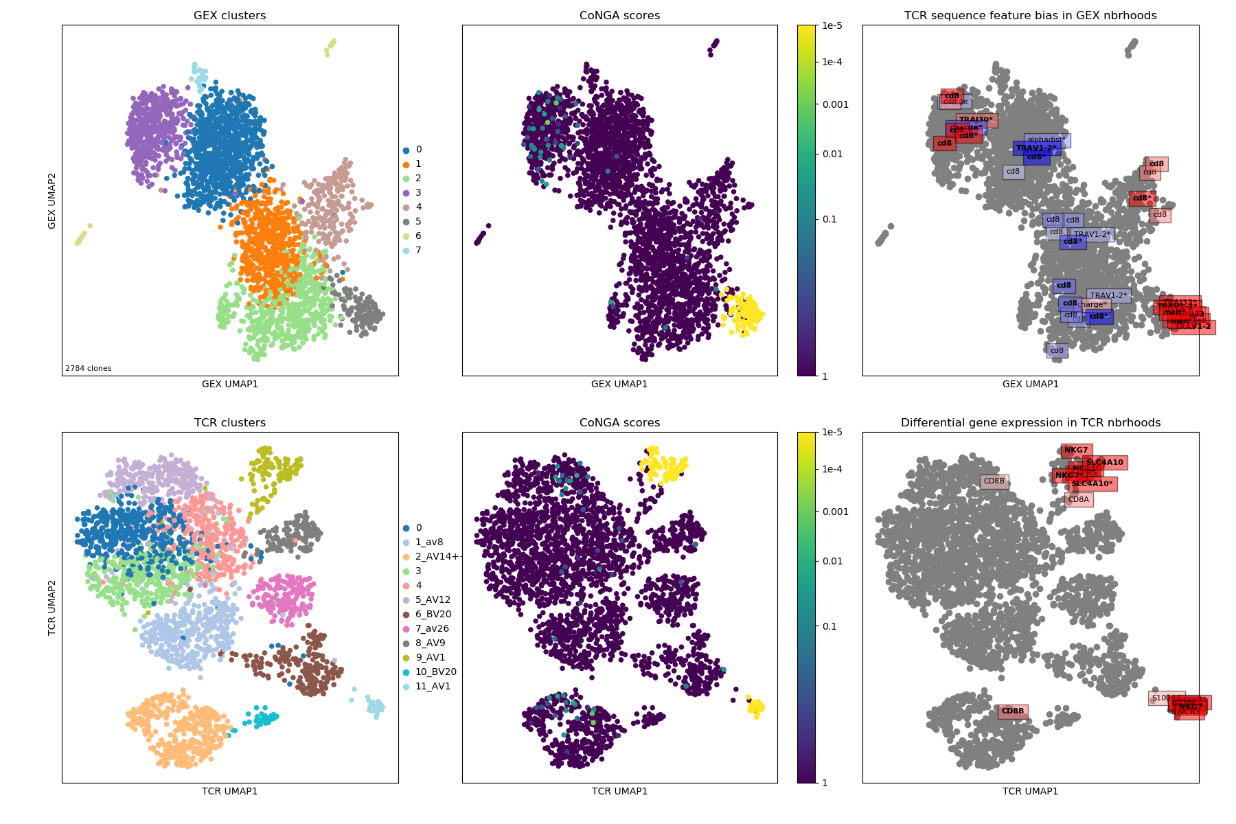
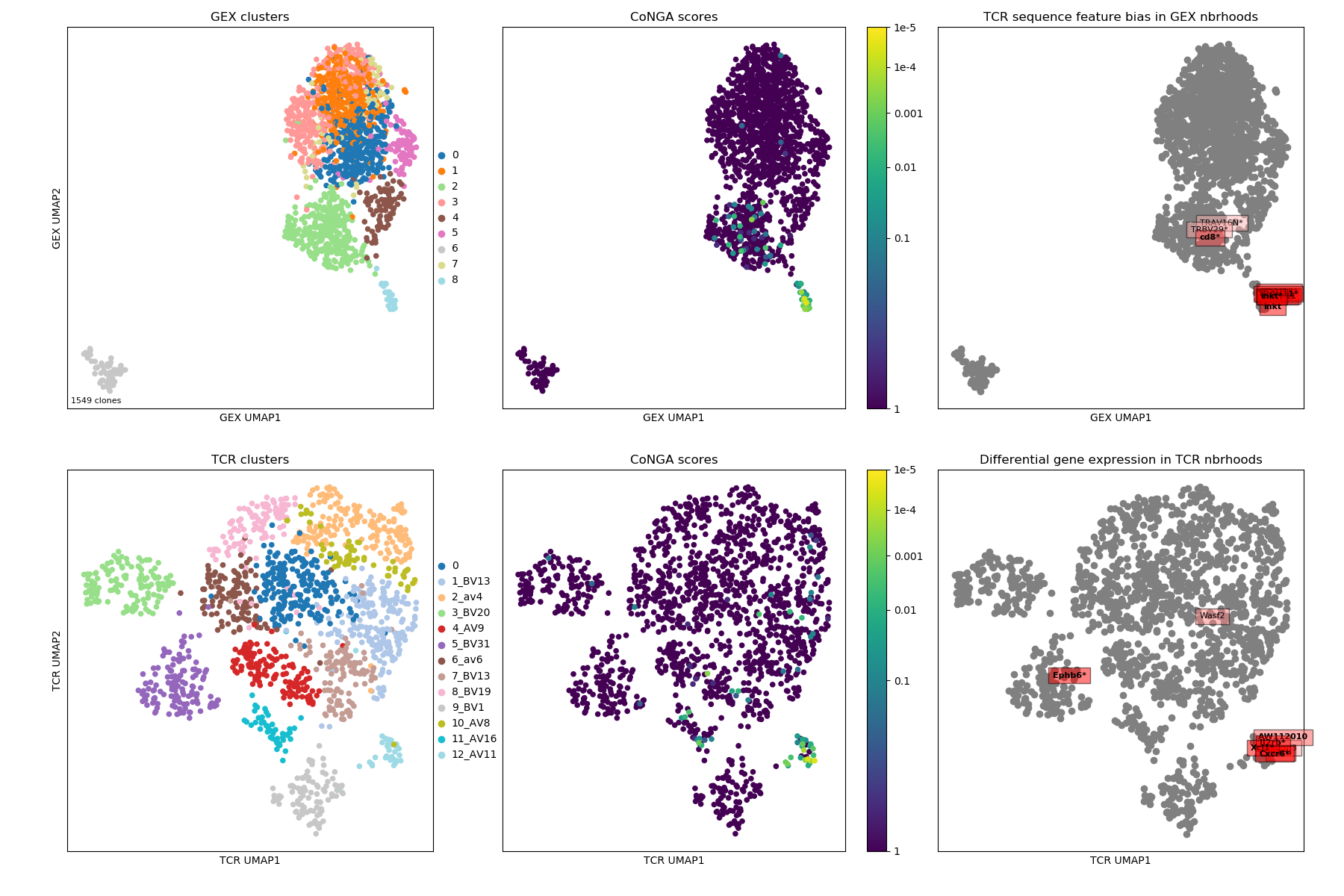
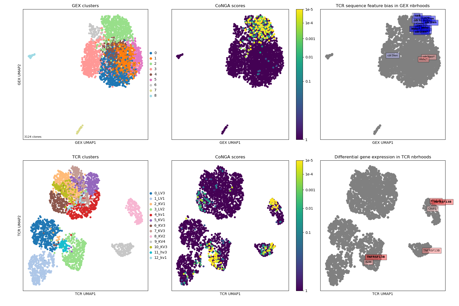
In looking at the CoNGA results a good place to start is with the summary image, which will be named something like OUTFILE_PREFIX_summary.png where OUTFILE_PREFIX was the --outfile_prefix command line argument passed to run_conga.py. This image shows 2D projections of the clonotypes in the dataset, based on distances in gene expression (GEX) space in the top row and in TCR/BCR space in the bottom row. The left panels are colored by clonotype clusters (GEX clusters on top and TCR clusters on the bottom); the middle panels are colored by CoNGA score, which reflects overlap between the GEX and TCR neighbor graphs on a per-clonotype basis; and the right panels are overlaid with the top graph-vs-feature hits: TCR features that are enriched in GEX graph neighborhoods on top, and genes that are differentially expressed in TCR graph neighborhoods on the bottom.

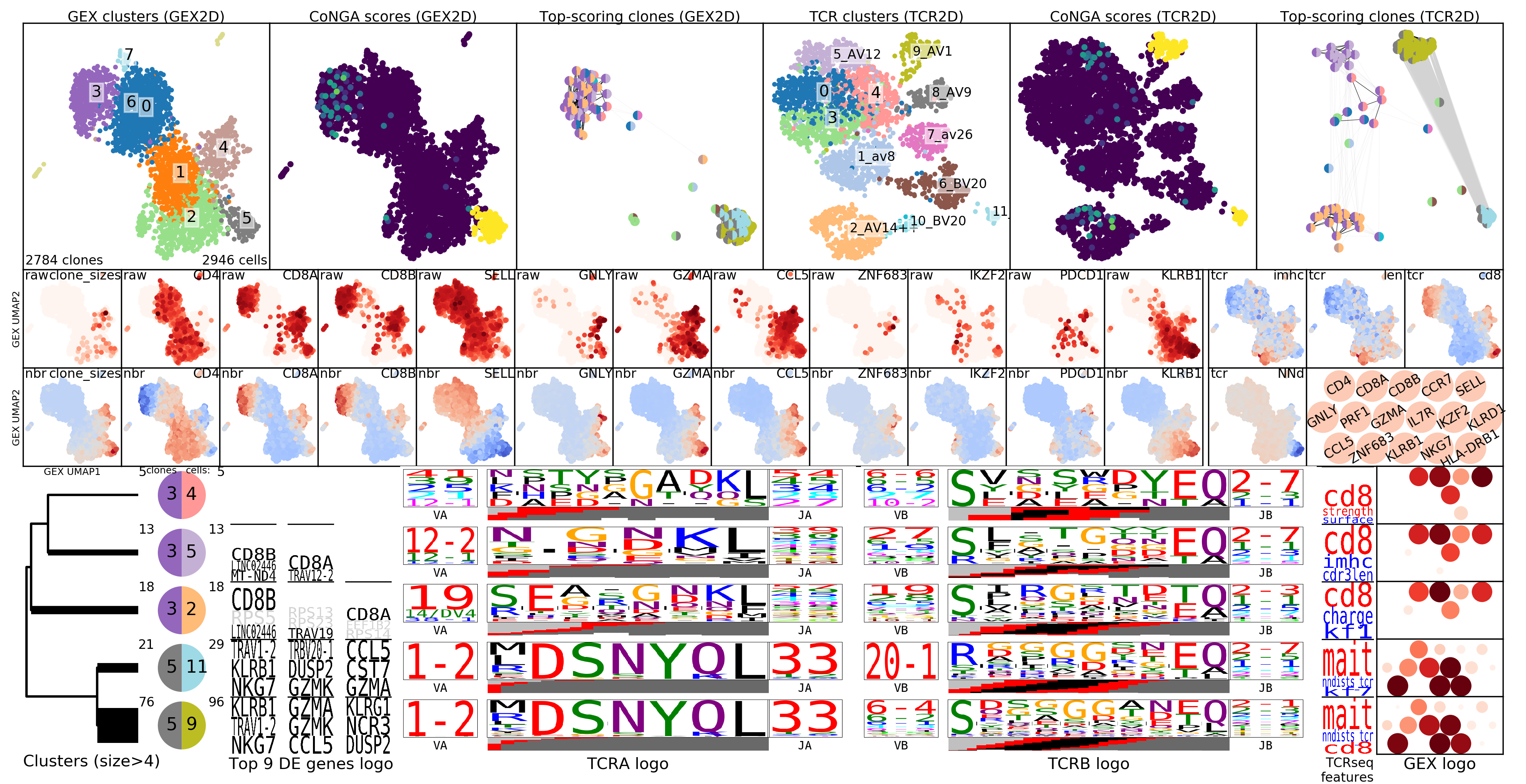
To gain greater insight into the clonotypes with significant CoNGA scores, the software groups them by their joint GEX and TCR cluster assignments and displays logos that summarize gene expression and TCR V/J gene usage and CDR3 sequence features for groups with size above a threshold (by default, at least 5 clonotypes and .1% of the overall dataset size). These logos are shown in the plot OUTFILE_PREFIX_bicluster_logos.png. In this image the top panels are show the clusters, conga scores, and conga hits (clonotypes with conga score<1) in the GEX (left 3 panels) and TCR/BCR (right 3 panels) 2D lanscapes. Below them are shown a sequence of thumbnail GEX projection scatter plots colored by selected (and user configurable) marker genes; the top set are colored by raw (normalized for cell reads and log+1 transformed) expression and in the bottom set those values are Z-standardized and averaged over GEX graph neighborhoods, to smooth and highlight overall trends. Below the snapshots are the rows of cluster-pair (or 'bicluster') logos.

The results of the graph-vs-features analysis are summarized in a number of graphs with names that include text like graph_vs_XXX_features. For example, the top few TCR/GEX feature hits are shown projected onto the other landscape (ie, TCR features onto the GEX landscape and GEX features onto the TCR landscape) in plots that end in _panels.png, like the OUTFILE_PREFIX_gex_nbr_graph_vs_tcr_features_panels.png shown below, where we can see MAIT-cell features as well as features that differ between CD4 and CD8 T cells (charge, TRBV20 and TRAJ30 usage). You can identify the CD4/CD8 cells by looking at the CD4/CD8a/CD8b gene thumbnails in the cluster logos plot above.

In addition to the graph-vs-feature analysis described in the preprint, we recently implemented a first, experimental version of the HotSpot method developed by the Yosef lab (bioRxiv preprint). Hotspot identifies numerical features that respect a given neighbor graph structure, so we can use it to identify GEX features that correlate with the TCR similarity graph and TCR/BCR features that correlate with the the GEX similarity graph. These features are saved to tsv files and visualized in a number of images, including seaborn clustermap plots if you have the seaborn package installed. For example the image with the rather long name OUTFILE_PREFIX_0.100_nbrs_combo_hotspot_features_vs_gex_clustermap_lessredundant.png shows the top combined GEX and TCR features (rows) versus clonotypes (columns), where the clonotypes (columns) are ordered based on a hierarchical clustering dendrogram built using GEX similarity (_vs_gex_clustermap in filename) and the scores are averaged over GEX neighborhoods (so that visible trends need to be consistent the GEX graph structure, and to smooth noise). Features that are highly correlated with another, more significant feature are filtered out and listed in the tiny blue text on the left (_lessredundant in the filename). In this plot we can see MAIT, CD4, and CD8 groupings and many of the same features as in the graph-vs-features analysis above. Since we have only implemented the simplest model right now, the P-values may not be completely trustworthy, and we suggest focusing on the results from larger neighbor graphs (here we are showing the results for the graph with 0.1 neighbor fraction, _0.100_nbrs in the filename, ie where each clonotype is connected to the nearest 10 percent of the dataset). The colors along the top of the matrix show the GEX cluster assignments of each clonotype. The two columns of colors along the left-hand side of the matrix show (left column) the P-value and (right column) the feature type (GEX vs TCR) of the feature corresponding to that row (P-values and feature types are also given in the row names along the right-hand side of the matrix). '[+N]' in the row name means that N additional highly-correlated features were filtered out; their names will be listed in the tiny blue text along the left-hand side of the figure, listed below the name of the representative feature. (Some of these images are big and very detailed-- downloading or opening in a separate tab and zooming in may be helpful).

Mouse PBMC dataset

# DOWNLOAD FROM:
# https://support.10xgenomics.com/single-cell-vdj/datasets/3.0.0/vdj_v1_mm_balbc_pbmc_5gex

# SETUP
/home/pbradley/anaconda2/envs/scanpy_new/bin/python /home/pbradley/gitrepos/conga/scripts/setup_10x_for_conga.py --organism mouse --filtered_contig_annotations_csvfile ./conga_example_datasets/vdj_v1_mm_balbc_pbmc_t_filtered_contig_annotations.csv

# RUN
/home/pbradley/anaconda2/envs/scanpy_new/bin/python /home/pbradley/gitrepos/conga/scripts/run_conga.py --all --organism mouse --clones_file ./conga_example_datasets/vdj_v1_mm_balbc_pbmc_t_filtered_contig_annotations_tcrdist_clones.tsv --gex_data ./conga_example_datasets/vdj_v1_mm_balbc_pbmc_5gex_filtered_gene_bc_matrices_h5.h5 --gex_data_type 10x_h5 --outfile_prefix tcr_mm_pbmc

The summary image, where we can see a tight cluster of conga hits that turn out to be iNKT cells (inkt TCR feature enriched in top right panel), some CD8-enriched genes (TRAV16N and TRBV29), and the EphB6 gene which turns out to be correlated with usage of the TRBV31 gene:

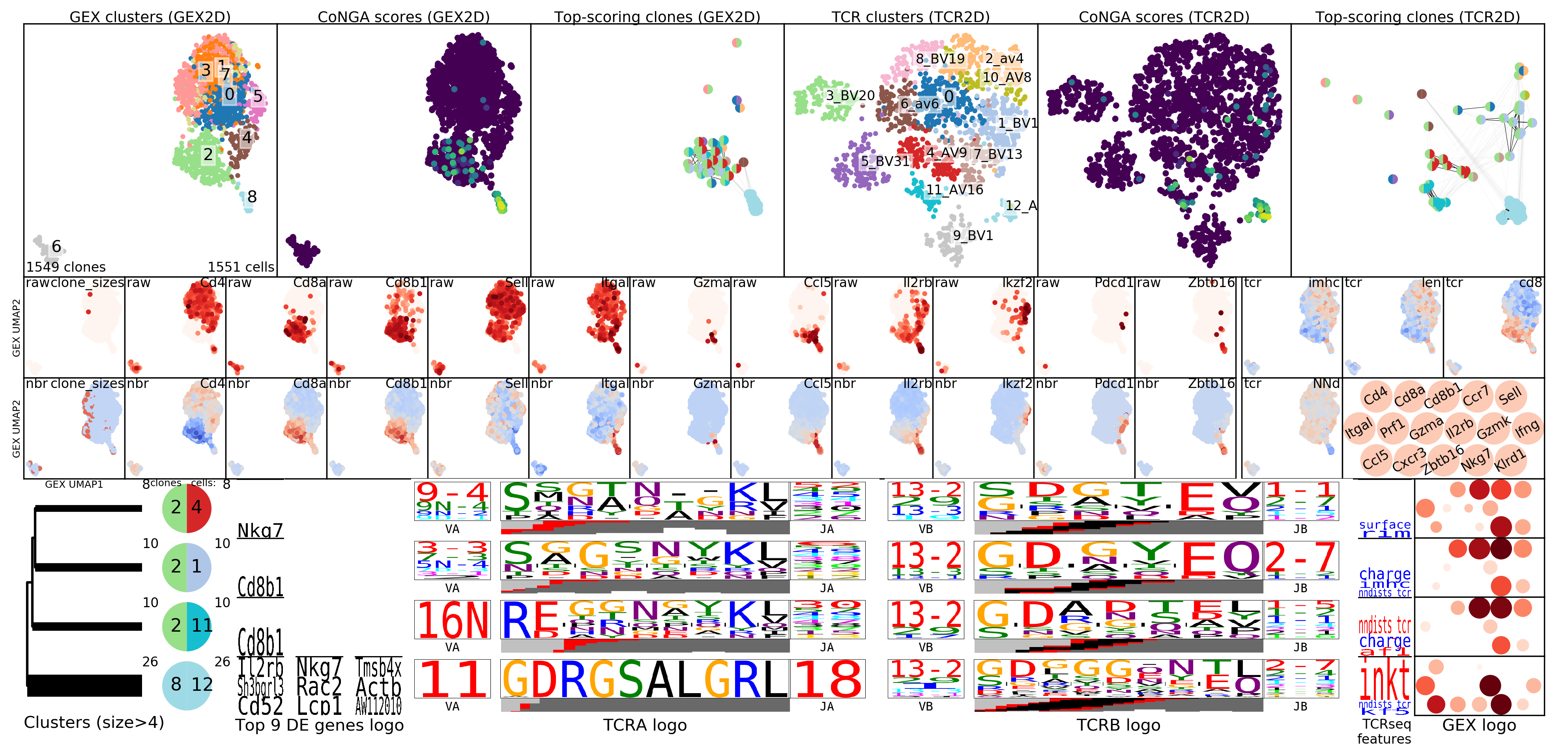
Here the cluster logo image shows iNKT cells and some CD8-positive clusters that likely reflect TCR sequence features shared by CD8s.

The top few GEX features that are enriched in TCR neighborhoods: some iNKT genes and the EphB6 gene showing localized expression in the TCR landscape projection (in the TRBV31 expressing clonotypes).

In the hotspot clustermap showing features versus TCR-arranged clonotypes we can see the correlation between EphB6 and TRBV31 nicely. The color rows along the top of the matrix show (from top to bottom) the TCR cluster assignment and the TRAV, TRAJ, TRBV, and TRBJ gene segment usage patterns (color key for the top few genes is shown at the top of the column dendrogram).

Human Melanoma B cell dataset

# DOWNLOAD FROM:
# https://support.10xgenomics.com/single-cell-vdj/datasets/4.0.0/sc5p_v1p1_hs_melanoma_10k

# SETUP
/home/pbradley/anaconda2/envs/scanpy_new/bin/python /home/pbradley/gitrepos/conga/scripts/setup_10x_for_conga.py --organism human_ig --filtered_contig_annotations_csvfile ./conga_example_datasets/sc5p_v1p1_hs_melanoma_10k_b_filtered_contig_annotations.csv --condense_clonotypes_by_tcrdist --tcrdist_threshold_for_condensing 50

# RUN
/home/pbradley/anaconda2/envs/scanpy_new/bin/python /home/pbradley/gitrepos/conga/scripts/run_conga.py --all --organism human_ig --clones_file ./conga_example_datasets/sc5p_v1p1_hs_melanoma_10k_b_filtered_contig_annotations_tcrdist_clones_condensed.tsv --gex_data ./conga_example_datasets/sc5p_v1p1_hs_melanoma_10k_filtered_feature_bc_matrix.h5 --gex_data_type 10x_h5 --outfile_prefix bcr_hs_melanoma

Two features to note in the commands above: (1) we are passing --organism human_ig to let conga know we are working with BCR data, (2) in the setup command we added the flags --condense_clonotypes_by_tcrdist --tcrdist_threshold_for_condensing 50, which trigger merging of 10X clonotypes whose TCRdist (actually BCR dist) is less than or equal to 50 (ie, we do single-linkage clustering and cut the tree at a distance threshold of 50). Here the goal is to merge clonally related families so that GEX/BCR covariation that we detect reflects the correlation across independent rearrangements. The user could instead apply a more sophisticated clone identification procedure and modify the raw_clonotype_id column in the contigs csv file, which is where conga gets the clonotype info.

The summary image, where we can see that most of the conga hits are in GEX cluster 2; that there are differences in CDR3 length across the landscape; and some specific genes that are differentially expressed in TCR graph neighborhoods (TNFRSF13B, B2M, CRIP1).

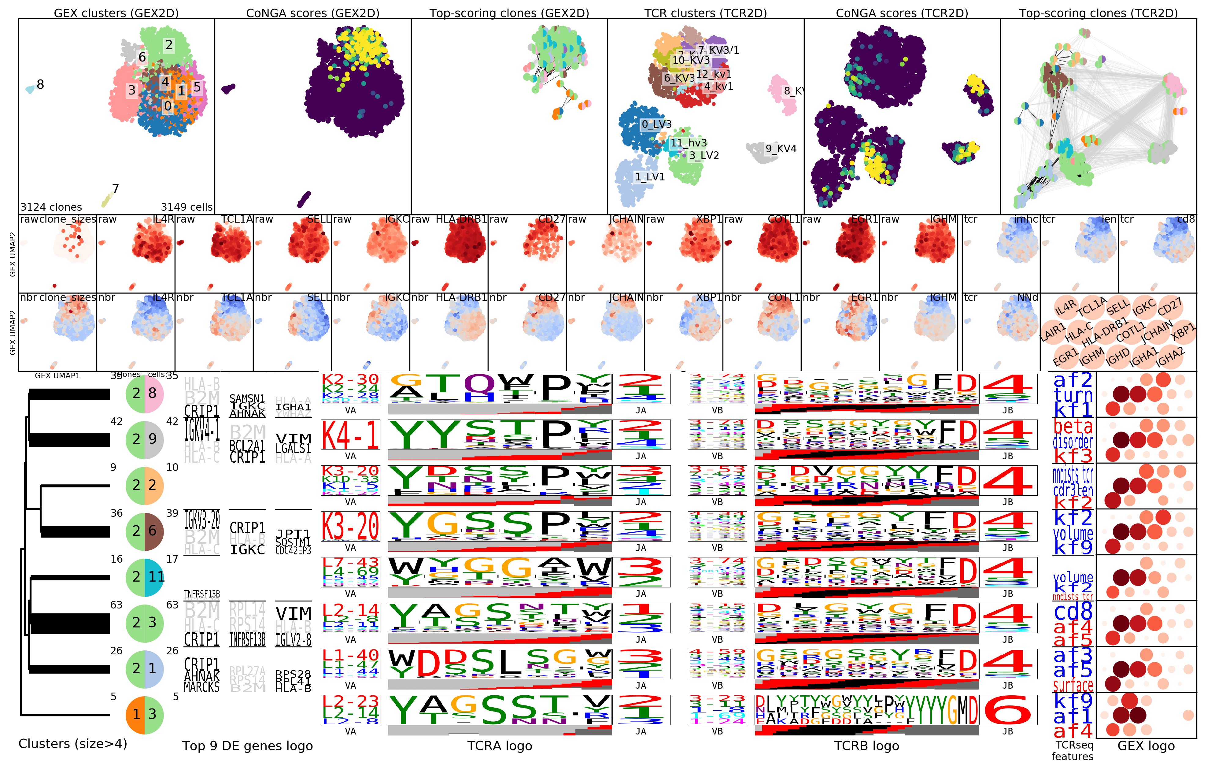
Logos for the clusters of conga hits, with one cluster of 'naive' clonotypes with long CDRH3s and high TCL1A expression.

In the hotspot clustermap showing features versus TCR-arranged clonotypes we can see a breakdown between naive and non-naive features, where IGHJ6 and CDR3 length are correlated with genes like TCL1A and class II HLA genes, and IGHJ4 is enriched in the non-naives.

CoNGA also makes a tree of all the clonotypes with a conga score less than a loose threshold value of 10, where we can look for sequence clustering. The branches are colored by a transformed version of the conga score that maps the threshold value of 10 to zero (blue) with more significant scores trending toward red at a value of 1e-8:

CoNGA data model: where stuff is stored

After setup, the conga package stores data in various locations in the scanpy AnnData object. Below we assume that adata is the name of the AnnData object where the GEX and TCR data is stored (this is the naming convention followed in CoNGA).

The core stuff

CoNGA functionality like graph-vs-graph and graph-vs-feature analyses will generally expect these to be set once the setup phase has completed. The CoNGA routines that fill these arrays are:

conga.preprocess.read_data: loads the GEX data into an AnnData object (here called adata); puts the TCR information into the adata.obs arrays; reads the TCRdist kernel principal components and stores them in adata.obsm under the key X_pca_tcr. Eliminates cells without paired TCR information.
conga.preprocess.filter_and_scale: sets up the adata.raw object, does some typical single-cell filtering and preprocessing.
conga.preprocess.reduce_to_single_cell_per_clone: reduces to a single cell per clonotype; fills the adata.obs['clone_sizes'] array and potentially adata.obsm[<batch_key>] for one or more <batch_key>s if there is batch structure defined in the input data.
conga.preprocess.cluster_and_tsne_and_umap: Fills adata.obsm['X_pca_gex'], and the adata.obs arrays X_gex_2d, X_tcr_2d, clusters_gex, and clusters_tcr.

`adata.obs`

The following 1-D arrays are stored in the obs array and can be accessed with expressions like adata.obs['va']

va: V gene names, alpha chain
ja: J gene names, alpha chain
cdr3a: CDR3 amino acid sequences, alpha chain
cdr3a_nucseq: CDR3 nucleotide sequences, alpha chain
vb: V gene names, beta chain
jb: J gene names, beta chain
cdr3b: CDR3 amino acid sequences, beta chain
cdr3b_nucseq: CDR3 nucleotide sequences, beta chain
clusters_gex: GEX cluster assignments, integers, range [0, num_clusters)
clusters_tcr: TCR cluster assignments, integers, range [0, num_clusters)
clone_sizes: The number of cells in each clonotype.

`adata.obsm`

The following multidimensional arrays are stored in the obsm array after setup.

X_pca_gex: The GEX principal components. Used for neighbor-finding, UMAP projections, etc.
X_pca_tcr: The TCRdist kernel principal components. May be missing if we are using the 'exact TCRdist neighbors' mode, which is useful for really big datasets where the kernel PCA calculation takes forever.
X_gex_2d: The 2D landscape projection based on GEX (UMAP by default).
X_tcr_2d: The 2D landscape projection based on TCR (UMAP by default).

`adata.uns`

These miscellaneous data are stashed in the adata.uns dictionary:

organism: A string indicating what type of TCR/BCR data is being analyzed. CoNGA currently supports the following choices:
- human: human alpha-beta TCRs
- mouse: mouse alpha-beta TCRs
- human_gd: human gamma-delta TCRs
- mouse_gd: mouse gamma-delta TCRs
- human_ig: human BCRs

`adata.raw`

This is where the raw data on gene expression is expected to live.

adata.raw.X Sparse matrix with the gene expression values for each gene. These will have been normalized to sum to 10,000 and then np.log1p'ed (had the natural logarithm taken after adding 1).
adata.raw.var_names The gene names; should match the number of columns in adata.raw.X.

GEX and TCR neighbors

Currently the neighborhood information is stored independently of the adata object, in a dictionary called all_nbrs. The keys of this dictionary are the neighborhood fractions aka nbr_fracs, floats that represent the size of the neighborhood as a fraction of the total number of clonotypes. The default nbr_fracs are [0.01, 0.1]. For each nbr_frac, all_nbrs[nbr_frac] = [gex_nbrs, tcr_nbrs] where gex_nbrs and tcr_nbrs are numpy arrays of shape (num_clonotypes,num_nbrs), and num_nbrs = int(nbr_frac*num_clonotypes). Note that a clonotype is not included in its own set of neighbors. Also note that the CoNGA neighbor information is distinct from neighbor information that scanpy uses for UMAP projection and clustering. CoNGA neighborhoods are larger than the neighborhoods typically used in clustering and dimensionality reduction.

Extras

This might be results of calculations that are stored for easier access, or optional data that is present in certain circumstances (for example when there are batches present). It should be OK if any of these are missing.

`adata.obs`

The following 1-D arrays are stored in the obs array and can be accessed with expressions like adata.obs['va']

is_invariant: Boolean array recording the presence of canonical invariant (MAIT or iNKT) TCR chains.
nndists_tcr: Nearest-neighbor distances based on TCR sequence. Gives an approximate measure of (inverse) TCR density.
nndists_gex: Nearest-neighbor distances based on GEX. Gives an approximate measure of (inverse) GEX density.
conga_scores: CoNGA scores for each clonotype. Filled after the graph-vs-graph analysis has been run.
<batch_key>: When there are multiple batches present in a dataset these can be tracked and visualized in many of the analysis and plotting routines. Here <batch_key> is the name of the batch/category (for example 'outcome' or 'subject' or 'timepoint'). The entry in adata.obs for each batch key should contain integers in the range [0,num_batch_classes). This information is stored in the adata.obs array prior to condensing to a single cell per clonotype, and in the adata.obsm array after condensing to a single cell per clonotype (since expanded clonotypes can span multiple batch assignments). See the FAQ entry on batches in CoNGA (coming soon).

`adata.obsm`

The following multidimensional arrays are stored in the obsm array and can be accessed with expressions like adata.obsm[<tag>]

<batch_key>: When there are multiple batches present in a dataset these can be tracked and visualized in many of the analysis and plotting routines. Here <batch_key> is the name of the batch/category (for example 'outcome' or 'subject' or 'timepoint'). For each <batch_key>, the array stored in adata.obsm should have shape (num_clonotypes,num_categories) where num_categories is the number of possible batch assignments. For example if there are three timepoints then num_categories for the 'timepoint' batch key would be 3. The (i,j) entry in the array will give the number of cells in clonotype i that were assigned to the batch assignment j. This array is filled automatically when we reduce to a single cell per clonotype, based on the information in the array adata.obs[<batch_key>] (see above). See the FAQ entry on batches in CoNGA (available soon).

`adata.uns`

batch_keys: A list of strings that gives the names of the different batch types/categories, if present (for example something like ['subject', 'outcome', 'timepoint']. For each name in adata.uns['batch_keys'] there should be an entry in the adata.obs array with that name (see above for description of that data). When we condense to a single cell per clonotype, we add an entry in the adata.obsm array with the same name, which contains the counts for each batch assignment summed over all the cells in each clonotype (so it's a 2D array and hence has to be stored in obsm not obs.

`adata.var`

feature_types: This array is used to detect and exclude antibody (site-seq) or other non-gene-expression features. If it's missing, then during setup CoNGA will assume that all the counts in the adata.X array are gene-expression features. The expected value for gene expression features in this array is the string 'Gene Expression'. CoNGA will look for and use any column in the adata.var array whose name starts with feature_types (since sometimes they get renamed during concatenation).

Frequently asked questions

My CoNGA docker process mysteriously stopped with the cryptic error message 'killed'
- You may need to increase the resources allocated to docker processes, in particular the memory. You could do this on the Resources tab of settings in the Docker desktop app. Or try a quick google search.
I get an error when I type import conga
- Note that this won't work automatically unless you used the pip install -e . installation method.
  - If you didn't, or that's not working for some reason, you can just manually add the conga github repository directory to your path before importing conga. For example:
```
import sys
path_to_conga = '/path/to/gitrepos/conga/' # contains README.md, scripts, conga
sys.path.append(path_to_conga)
import conga
```
How can I visualize the different batches in my data? Or other discrete/categorical features assigned to individual cells? Right now, CoNGA has a simple framework for analyzing this kind of data. There can be multiple flavors of "batch" information, like donor, tissue, disease, etc. Each must be represented as an integer-valued column in adata.obs, and the names of the different batch columns should be given as a list in adata.uns['batch_keys'].

One easy way to add these columns is through the scripts/merge_samples.py script, which accepts a --batch_keys argument. That argument should be a list of column names where those columns are present in the samples tsvfile provided with the --samples argument. So if you are merging data and the batch structure you want to visualize breaks down by the input files, that should work.

For more complicated data, the best thing is to read the GEX data into a scanpy AnnData object and manually add the new batch columns to the adata.obs array. Then save the new AnnData for analyzing with scripts/run_conga.py or a jupyter notebook.

For example, something like this:
```
import scanpy as sc
import pandas as pd

old_gex_filename = 'filtered_gene_bc_matrices.h5'
new_gex_filename = 'filtered_gene_bc_matrices_w_batches.h5ad'

# has columns: barcode donor sample tissue
batch_info_tsvfile = 'cell_batch_info.tsv'

adata = sc.read_10x_h5(old_gex_filename)
batch_info = pd.read_csv(batch_info_tsvfile, sep='\t')
batch_info.set_index('barcode', drop=True, inplace=True)

df = adata.obs.join(batch_info) # funny behavior if I try to reassign adata.obs
for col in batch_info:
  adata.obs[col] = df[col]
adata.uns['batch_keys'] = list(batch_info.columns)

adata.write_h5ad(new_gex_filename)
```
When using run_conga.py to analyze data with batches, provide the adata.obs batch column names with the argument --batch_keys.

This functionality is still under development. Let us know if you run into any trouble.
I have a question that isn't addressed here. What should I do?
- You could open an issue on github, or email Phil and Stefan (emails at the top of this README) and we will try to help.

Dongfang1021/conga

Clonotype Neighbor Graph Analysis (CoNGA) -- version 0.1.1

Table of Contents

Running

Installation

Overview

Details

Even more details

Migrating Seurat data to CoNGA

Merging multiple datasets into a single object for CoNGA analysis

Updates

svg to png

Testing CoNGA without going through the pain of installing it

Docker

Google colab

Examples

Human PBMC dataset

Mouse PBMC dataset

Human Melanoma B cell dataset

CoNGA data model: where stuff is stored

The core stuff

`adata.obs`

`adata.obsm`

`adata.uns`

`adata.raw`

GEX and TCR neighbors

Extras

`adata.obs`

`adata.obsm`

`adata.uns`

`adata.var`

Frequently asked questions