The Land Variational Ensemble Data Assimilation fRamework (LaVEnDAR) implements the method of Four-Dimensional Ensemble Variational data assimilation for land surface models. In this README we show an example of implementing 4DEnVar with the JULES land surface model.
The data assimilation routines and minimization are included in fourdenvar.py. For the example included in this
project you will require an installation of the JULES land surface model (more information on JULES can be found here:
https://jules.jchmr.org/ ). Model specific routines for running JULES are found in jules.py and
run_jules.py. The data assimilation experiment is setup in experiment_setup.py with variables set for
output directories, model parameters, ensemble size and functions to extract observations for assimilation. The module
run_experiment.py runs the ensemble of model runs and executes the experiment as defined by
experiment_setup.py. Some experiment specific plotting routines are also included in plot.py.
Data for running the JULES model can be found in the data/ directory, including driving data for the Mead maize
FLUXNET site, a JULES dump file and a JULES land fraction file. There are 2 JULES namelist file directories
example_nml and williams_nml. The example_nml directory is used for JULES runs in the example
experiment included in the tutorial. The williams_nml directory was used to produce a "model truth" JULES run
from which pseudo observations are sampled in the tutorial example. Output from the different JULES model runs are
stored in the various subdirectories under the output/ directory.
This module controls how the experiment will be run. Output and namelist directories are set by output_directory
and nml_directory. The model executable path is set by model_exe. The functions to exatract the mean
prior model estimate to the assimilated observations, the ensemble of prior estimates to the observations and the
assimilated observations are set by jules_hxb, jules_hxb_ens and obs_fn respectively. These
functions are defined in the observations.py module and are experiment and model specific.
The parameters to be optimised in the experiment are set in the dictionary opt_params, in the tutorial
experiment the dictionary is defined as:
opt_params = {'pft_params': {
                  'jules_pftparm': {
                      'neff_io': [7, 6.24155040e-04, (5e-05, 0.0015)],
                      'alpha_io': [7, 6.73249126e-02, (0, 1.0)],
                      'fd_io': [7, 8.66181324e-03, (0.0001, 0.1)]}},
              'crop_params': {
                  'jules_cropparm': {
                      'gamma_io': [2, 2.07047321e+01, (0.0, 40.0)],
                      'delta_io': [2, -2.97701647e-01, (-2.0, 0.0)],
                      'mu_io': [2, 2.37351160e-02, (0.0, 1.0)],
                      'nu_io': [2, 4.16006288e+00, (0.0, 20.0)]}}}
where each heading in the opt_params dictionary corresponds to a JULES namelist filename and contains another
dictiontary for the JULES namelists defined within that file. Each namelist heading contains a dictionary of the
parameters to change within the namelist. The parameters hold a list of size 3 containing the index of
the parameter to be optimised, the prior value to use for the parameter and the bounds (low, high) for the parameter.
For example if we want to optimise the value of nitrogen use efficiency (neff_io) for maize in JULES we have to
first specify the filename where this parameter appears pft_params. Then in the dictionary below
pft_params specify the namelist where the parameter appears jules_pftparm. Then in the dictionary below
jules_pftparm specify neff_io with a list of the maize plant functional type index, its prior value and
its bounds.
We specify the error set on the prior parameters with prior_err, the ensemble size with
ensemble_size, the number of processors to use for the experiment with num_processes and the seed value
for any random perturbations performed in the experiment with seed_value. We also set a function to save
plotting output from the data assimilation experiments with save_plots and a save directory with
plot_output_dir.
In this tutorial we run a twin experiment to recover 7 JULES model parameters from a known model truth. The tutorial
focuses on the maize plant functional type within JULES-crop. We assimilate observations of for leaf area index, gross
primary productivity and canopy height sampled from a "model truth". These are similar to the observations we expect to
have for real site level data. The functions used to extract these observations and the JULES modelled estimate to these
observations are included in observations.py. The rest of the setup can be seen within experiment_setup.py.
Note
To run this tutorial you must have a version of JULES installed on your system. The path to the executable for your
version of JULES must be included in the model_exe variable in experiment_setup.py.
Once the variables in experiment_setup.py have been set it is possbile to run the default data assimilation
experiment by moving into the lavendar/ directory and running the command:
python run_experiment.py run_xb run_xa plot
This will run the full example data assimilation experiment, with the run_xb argument running the prior mean
JULES model, run_xa running the analysis ensemble after the data assimilation has been performed and
plot saving plotting output from the save_plots function in experiment_setup.py.
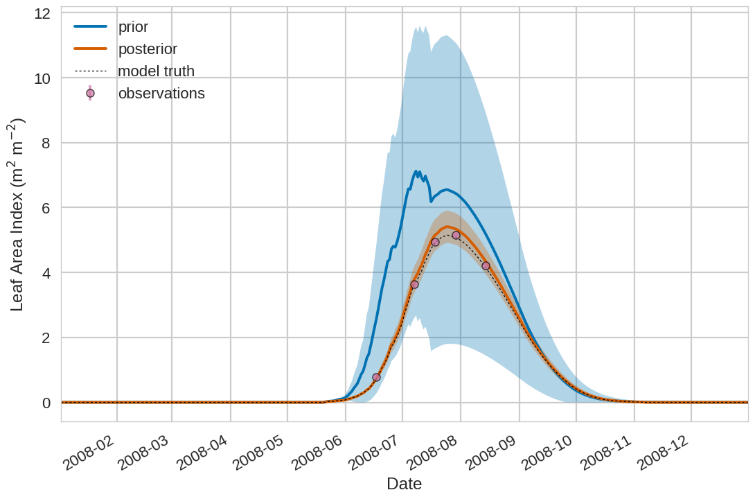
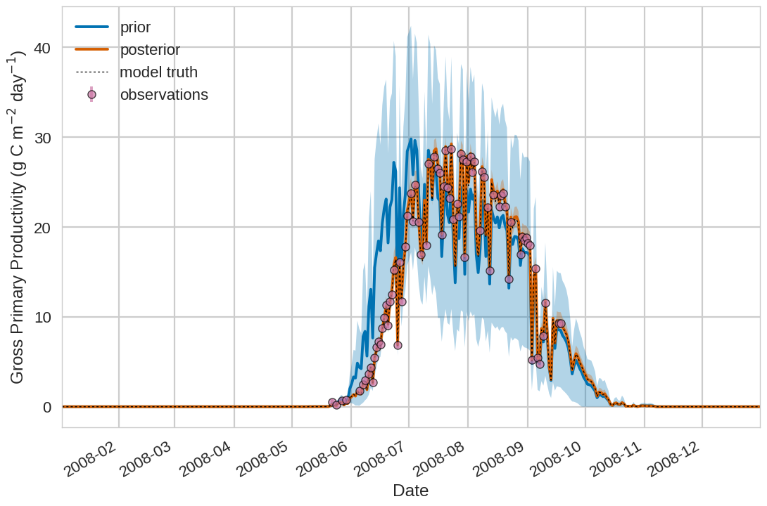
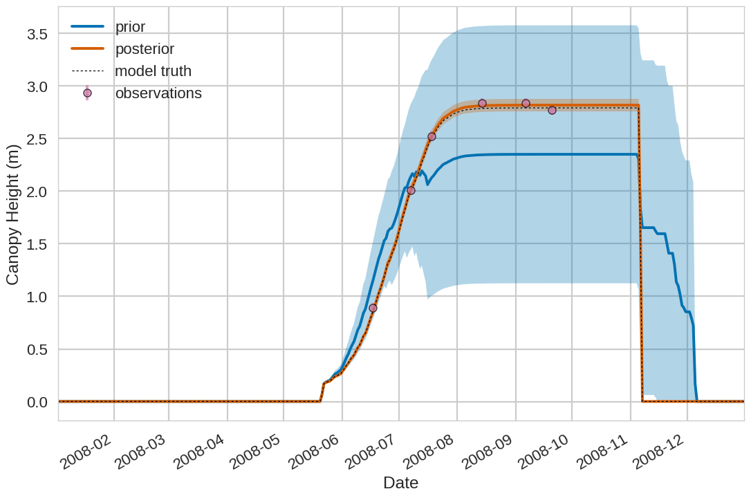
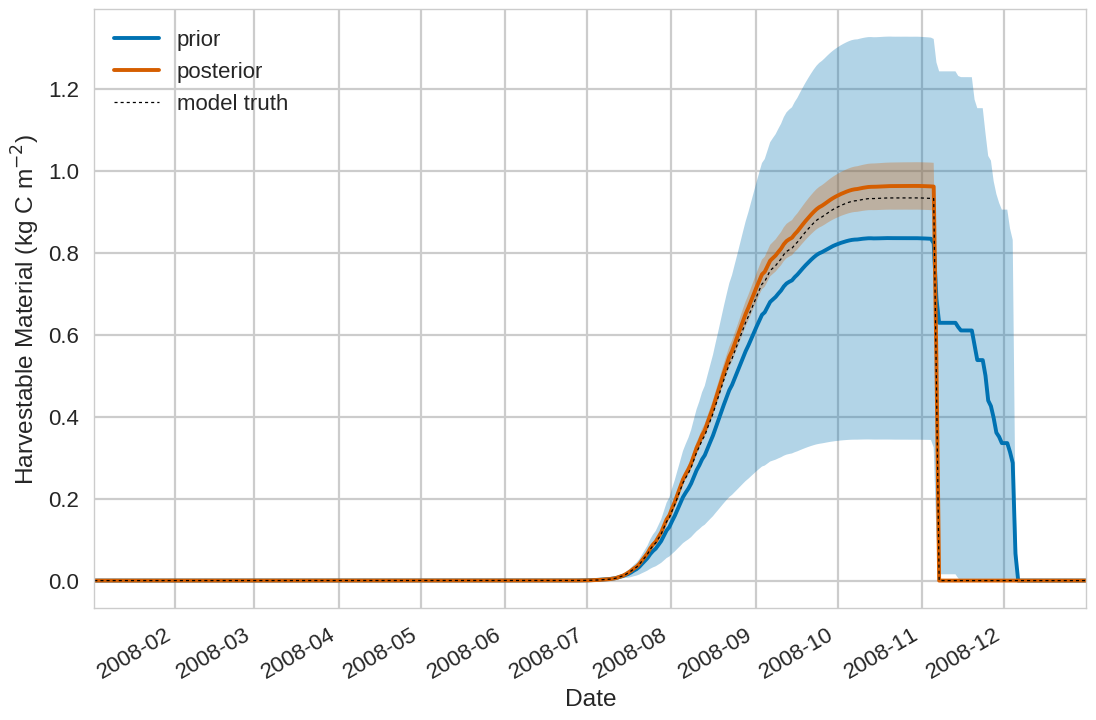
Below we include the example plotting output from the tutorial exercise. For the first 4 plots below the Blue shading is
the prior ensemble spread (+/- 1 standard deviation), the orange shading is the posterior ensemble spread
(+/- 1 standard deviation), the pink dots are observations with error bars and the dashed black line is the model truth.
For all variables (including unobserved harvestable material) we can see we are much closer to the truth with the
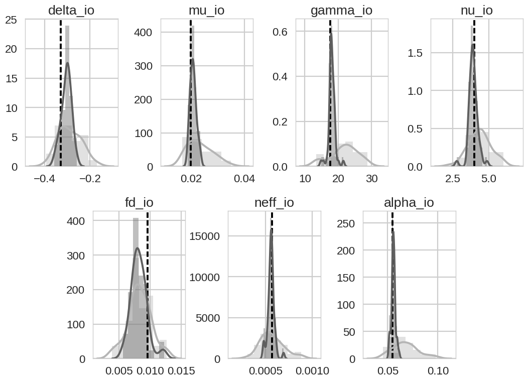
posterior estimate after data assimilation. Prior and posterior distributions for the 7 optimised parameters are shown
in the final plot where light grey is the prior distribution, dark grey is the posterior distribution and the black
dashed line is the model truth value. We can see that for this experiment all model parameters shift towards the model
truth, except for the scale factor for dark respiration fd_io. This is due to the fact that the
assimilated observations are not giving any constraint on the dark respiration of the plant as all observations are
averaged daily and we only have gross primary productivity and not net primary productivity. The parameters being
optimised in this experiment can be changed in the opt_params dictionary in experiment_setup.py, make
sure the index set in the opt_params dictionary is for the the plant functional type that is being observed.
In the case of any issues or inquiries please contact: e.pinnington@reading.ac.uk
