Neural networks, especially deep neural networks with many parameters, require a large amount of training data. This has led to the development of sophisticated data augmentation methods as well as entire industries dedicated to data annotation. The validation of these annotation labels is a common problem whenever such a large amount of data is involved as incorrect, or noisy, labels can lead to incorrectly trained machine learning algorithms that do not properly identify patterns within the data.
All code can be found on the Github repository, Learning with Noisy Labels.
# Ensure reproducible results
import numpy as np
np.random.seed(101)
import tensorflow
tensorflow.set_random_seed(101)
import pandas as pd
import h5py
import matplotlib.pyplot as plt
%matplotlib inline
import sklearn.model_selection
import sklearn.metrics
import keras.utils
import keras.datasets
from keras.models import Model
from keras.layers import Input, Conv2D, MaxPool2D, Dense, Flatten
Using TensorFlow backend.
To showcase the effects of noisy labels, I will use the MNIST handwritten digit dataset.
(x_train, y_train), (x_test, y_test) = keras.datasets.mnist.load_data()

# Min-Max Scaling
train_min = np.min(x_train, axis=(1, 2))[:, np.newaxis, np.newaxis]
train_max = np.max(x_train, axis=(1, 2))[:, np.newaxis, np.newaxis]
x_train = (x_train - train_min) / (train_max - train_min)
test_min = np.min(x_test, axis=(1, 2))[:, np.newaxis, np.newaxis]
test_max = np.max(x_test, axis=(1, 2))[:, np.newaxis, np.newaxis]
x_test = (x_test - test_min) / (test_max - test_min)

# Transform input to be 4D
x_train = x_train[..., None]
x_test = x_test[..., None]
The images are stored as a 4D array (Tensorflow format: batch size, width, height, number of channels) and the labels are a simple 1D array.
print("Training Images array shape: {}".format(x_train.shape))
print("Testing Images array shape:  {}".format(x_test.shape))
print("Training Labels array shape: {}".format(y_train.shape))
print("Testing Labels array shape:  {}".format(y_test.shape))
Training Images array shape: (60000, 28, 28, 1)
Testing Images array shape: (10000, 28, 28, 1)
Training Labels array shape: (60000,)
Testing Labels array shape: (10000,)
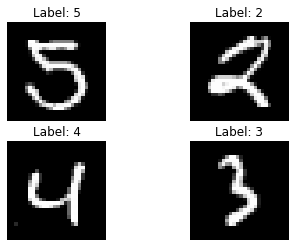
A look at some of the digits shows us the expected output.
fig, ax = plt.subplots(2, 2);
ax[0, 0].imshow(x_train[284, ..., 0], cmap="gray");
ax[0, 0].set_title("Label: " + str(y_train[284]));
ax[0, 0].axis("off");
ax[0, 1].imshow(x_train[1129, ..., 0], cmap="gray");
ax[0, 1].set_title("Label: " + str(y_train[1129]));
ax[0, 1].axis("off");
ax[1, 0].imshow(x_test[9471, ..., 0], cmap="gray");
ax[1, 0].set_title("Label: " + str(y_test[9471]));
ax[1, 0].axis("off");
ax[1, 1].imshow(x_test[44, ..., 0], cmap="gray");
ax[1, 1].set_title("Label: " + str(y_test[44]));
ax[1, 1].axis("off");
plt.show()I'll be using a simple convolutional network for this task. MNIST is an extremely easy dataset to classify and doesn't require a particularly sophisticated model.
def get_model(img_shape, nclasses):
    """
    Build convolutional network
    :param img_shape:
    :param nclasses:
    :return:
    """
    inputs = Input(shape=img_shape, name="Input")
    conv1 = Conv2D(
        filters=32, kernel_size=(3, 3),
        activation="relu", padding="valid",
        strides=(1, 1), name="Conv1")(inputs)
    conv2 = Conv2D(
        filters=32, kernel_size=(3, 3),
        activation="relu", padding="valid",
        strides=(1, 1), name="Conv2")(conv1)
    maxpool1 = MaxPool2D(
        pool_size=(3, 3), strides=(2, 2),
        padding="valid", name="MaxPool1")(conv2)

    conv3 = Conv2D(
        filters=64, kernel_size=(3, 3),
        activation="relu", padding="valid",
        strides=(1, 1), name="Conv3")(maxpool1)
    conv4 = Conv2D(
        filters=64, kernel_size=(3, 3),
        activation="relu", padding="valid",
        strides=(1, 1), name="Conv4")(conv3)
    maxpool2 = MaxPool2D(
        pool_size=(3, 3), strides=(2, 2),
        padding="valid", name="MaxPool2")(conv4)

    flattened = Flatten(name="Reshape")(maxpool2)

    outputs = Dense(name="Dense", units=nclasses, activation="sigmoid")(flattened)

    model = Model(inputs=inputs, outputs=outputs)
    model.compile(loss="categorical_crossentropy", optimizer="Adam")

    return model
model = get_model(
img_shape=x_train.shape[1:4],
nclasses=len(np.unique(y_train)))WARNING:tensorflow:From /home/jan/anaconda3/envs/py3/lib/python3.7/site-packages/tensorflow/python/framework/op_def_library.py:263: colocate_with (from tensorflow.python.framework.ops) is deprecated and will be removed in a future version.
Instructions for updating:
Colocations handled automatically by placer.
def print_model(model):
    desc = "Name      | Output Shape        | Kernel / Pool Shape\n"
    desc += "----------|---------------------|--------------------\n"
    for layer in model.layers:
        desc += "{:<10}|".format(layer.name)
        desc += " {:<20}|".format(str(layer.output_shape))
        if hasattr(layer, "kernel"):
            desc += " {:<20}".format(str(layer.kernel.shape.as_list()))
        if hasattr(layer, "pool_size"):
            desc += " {:<20}".format(str(layer.pool_size))
        desc += "\n"
    print(desc)

print_model(model)
Name | Output Shape | Kernel / Pool Shape
----------|---------------------|--------------------
Input | (None, 28, 28, 1) |
Conv1 | (None, 26, 26, 32) | [3, 3, 1, 32]
Conv2 | (None, 24, 24, 32) | [3, 3, 32, 32]
MaxPool1 | (None, 11, 11, 32) | (3, 3)
Conv3 | (None, 9, 9, 64) | [3, 3, 32, 64]
Conv4 | (None, 7, 7, 64) | [3, 3, 64, 64]
MaxPool2 | (None, 3, 3, 64) | (3, 3)
Reshape | (None, 576) |
Dense | (None, 10) | [576, 10]
Next, I want to define a function that scrambles the labels. It's important that this function allows us to control the fraction of labels that are guaranteed to be correct. That means labels selected for scrambling may not get their original label assigned to them.
def scramble_labels(labels, percentage, possible_values=None):
    """
    Takes a label vector and randomly scrambles a fraction of the labels.

    The scrambling ensures that none of the altered labels will have their
    original value, i.e. the scrambling percentage is guaranteed.

    By default, the function assumes that 'labels' contains all possible
    label values. Should this not be the case, 'possible_values' can be used
    to pass a list of all possible labels.

    :param labels: Numpy array (num_labels,)
    :param percentage: Integer
    :param possible_values: Numpy array (num_unique_labels,)
    :return:
    """
    if percentage > 1:
        print("'scramble_freq' truncated to 1.0")
        percentage = 1.0

    if percentage == 0:
        return labels

    labels = labels.flatten()

    labels_to_scramble = np.random.choice(
        a=range(len(labels)),
        size=int(len(labels) * percentage),
        replace=False)

    # Define possible values for each entry
    if possible_values is None:
        possible_values = np.unique(labels)

    if not np.all(np.isin(np.unique(labels), possible_values)):
        raise ValueError(
            "'labels' contains values not found in 'possible_values'")

    possible_values = np.repeat(
        a=np.expand_dims(possible_values, 0),
        repeats=labels_to_scramble.shape[0],
        axis=0)
    forbidden_values = np.repeat(
        a=np.expand_dims(labels[labels_to_scramble], 1),
        repeats=len(np.unique(labels)), axis=1)

    sel = possible_values != forbidden_values
    new_possible_values = np.reshape(
        a=possible_values[sel],
        newshape=(possible_values.shape[0], possible_values.shape[1]-1))

    new_values = []
    for vals in new_possible_values:
        new_values.append(np.random.choice(vals))
    new_values = np.array(new_values)
    labels[labels_to_scramble] = new_values

    return labels
I can test this function with a dummy example:
dummy_labels = np.arange(10)
print("Original labels: {}".format(dummy_labels))
print("10% scrambling:  {}".format(scramble_labels(dummy_labels, 0.1)))
print("50% scrambling:  {}".format(scramble_labels(dummy_labels, 0.5)))
print("100% scrambling: {}".format(scramble_labels(dummy_labels, 1)))
Original labels: [0 1 2 3 4 5 6 7 8 9]
10% scrambling: [0 6 2 3 4 5 6 7 8 9]
50% scrambling: [0 1 2 3 9 3 8 8 8 0]
100% scrambling: [5 9 7 8 8 2 8 8 0 4]
To assess the model's performance, I train the model on the scrambled labels but then assess its performance with regards to the true labels to ascertain how well it reconstructs the correct relationship between input data and true labels from the noisy training data. A comparison of the training and validation losses shows that the models are not overfitting.
f1scores_real = []
f1scores_scrambled = []
training_histories = []
percentages = np.arange(0, 1.1, 0.1)

for p in percentages:
    print("Scrambling percentage: {:.2f}".format(p))
    print("-------------------------")
    y_train_scrambled = scramble_labels(
        labels=y_train, percentage=p)
    y_test_scrambled = scramble_labels(
        labels=y_test, percentage=p)

    y_train_cat = keras.utils.to_categorical(y_train)
    y_test_cat = keras.utils.to_categorical(y_test)
    y_train_scrambled_cat = keras.utils.to_categorical(y_train_scrambled)
    y_test_scrambled_cat = keras.utils.to_categorical(y_test_scrambled)

    training_histories.append(model.fit(
        x=x_train, y=y_train_scrambled_cat,
        validation_split=0.3,
        batch_size=32, epochs=5, verbose=2))

    pred = model.predict(x=x_test)

    f1scores_real.append(
        sklearn.metrics.f1_score(
            y_true=np.argmax(y_test_cat, axis=1),
            y_pred=np.argmax(pred, axis=1),
            average="weighted"))

    f1scores_scrambled.append(
        sklearn.metrics.f1_score(
            y_true=np.argmax(y_test_scrambled_cat, axis=1),
            y_pred=np.argmax(pred, axis=1),
            average="weighted"))
    print("-------------------------")
Scrambling percentage: 0.0
-------------------------
WARNING:tensorflow:From /home/jan/anaconda3/envs/py3/lib/python3.7/site-packages/tensorflow/python/ops/math_ops.py:3066: to_int32 (from tensorflow.python.ops.math_ops) is deprecated and will be removed in a future version.
Instructions for updating:
Use tf.cast instead.
Train on 42000 samples, validate on 18000 samples
Epoch 1/5
- 24s - loss: 0.1859 - val_loss: 0.0789
Epoch 2/5
- 32s - loss: 0.0526 - val_loss: 0.0592
Epoch 3/5
- 25s - loss: 0.0420 - val_loss: 0.0447
Epoch 4/5
- 24s - loss: 0.0318 - val_loss: nan
Epoch 5/5
- 44s - loss: 0.0276 - val_loss: 0.0534
-------------------------
Scrambling percentage: 0.1
-------------------------
Train on 42000 samples, validate on 18000 samples
Epoch 1/5
- 44s - loss: 0.6467 - val_loss: 0.6239
Epoch 2/5
- 46s - loss: 0.6051 - val_loss: 0.6141
Epoch 3/5
- 43s - loss: 0.5853 - val_loss: 0.6141
Epoch 4/5
- 44s - loss: 0.5683 - val_loss: 0.6179
Epoch 5/5
- 44s - loss: 0.5520 - val_loss: 0.6262
-------------------------
Scrambling percentage: 0.2
-------------------------
Train on 42000 samples, validate on 18000 samples
Epoch 1/5
- 46s - loss: 1.0086 - val_loss: 1.0217
Epoch 2/5
- 43s - loss: 0.9779 - val_loss: 1.0161
Epoch 3/5
- 41s - loss: 0.9581 - val_loss: 1.0198
Epoch 4/5
- 41s - loss: 0.9394 - val_loss: 1.0240
Epoch 5/5
- 41s - loss: 0.9164 - val_loss: 1.0423
-------------------------
Scrambling percentage: 0.30000000000000004
-------------------------
Train on 42000 samples, validate on 18000 samples
Epoch 1/5
- 42s - loss: 1.3353 - val_loss: 1.3507
Epoch 2/5
- 43s - loss: 1.3038 - val_loss: 1.3353
Epoch 3/5
- 41s - loss: 1.2841 - val_loss: 1.3420
Epoch 4/5
- 41s - loss: 1.2636 - val_loss: 1.3597
Epoch 5/5
- 38s - loss: 1.2394 - val_loss: 1.3804
-------------------------
Scrambling percentage: 0.4
-------------------------
Train on 42000 samples, validate on 18000 samples
Epoch 1/5
- 23s - loss: 1.6106 - val_loss: 1.6083
Epoch 2/5
- 23s - loss: 1.5787 - val_loss: 1.6086
Epoch 3/5
- 23s - loss: 1.5578 - val_loss: 1.6170
Epoch 4/5
- 23s - loss: 1.5367 - val_loss: 1.6221
Epoch 5/5
- 23s - loss: 1.5085 - val_loss: 1.6413
-------------------------
Scrambling percentage: 0.5
-------------------------
Train on 42000 samples, validate on 18000 samples
Epoch 1/5
- 23s - loss: 1.8464 - val_loss: 1.8496
Epoch 2/5
- 23s - loss: 1.8199 - val_loss: 1.8432
Epoch 3/5
- 23s - loss: 1.8008 - val_loss: 1.8426
Epoch 4/5
- 23s - loss: 1.7802 - val_loss: 1.8527
Epoch 5/5
- 23s - loss: 1.7537 - val_loss: 1.8637
-------------------------
Scrambling percentage: 0.6000000000000001
-------------------------
Train on 42000 samples, validate on 18000 samples
Epoch 1/5
- 23s - loss: 2.0305 - val_loss: 2.0313
Epoch 2/5
- 23s - loss: 2.0070 - val_loss: 2.0300
Epoch 3/5
- 23s - loss: 1.9887 - val_loss: 2.0411
Epoch 4/5
- 23s - loss: 1.9686 - val_loss: 2.0470
Epoch 5/5
- 26s - loss: 1.9439 - val_loss: 2.0600
-------------------------
Scrambling percentage: 0.7000000000000001
-------------------------
Train on 42000 samples, validate on 18000 samples
Epoch 1/5
- 23s - loss: 2.1786 - val_loss: 2.1752
Epoch 2/5
- 23s - loss: 2.1614 - val_loss: 2.1752
Epoch 3/5
- 23s - loss: 2.1467 - val_loss: 2.1788
Epoch 4/5
- 23s - loss: 2.1309 - val_loss: 2.1865
Epoch 5/5
- 23s - loss: 2.1086 - val_loss: 2.2018
-------------------------
Scrambling percentage: 0.8
-------------------------
Train on 42000 samples, validate on 18000 samples
Epoch 1/5
- 23s - loss: 2.2729 - val_loss: 2.2690
Epoch 2/5
- 23s - loss: 2.2623 - val_loss: 2.2690
Epoch 3/5
- 23s - loss: 2.2546 - val_loss: 2.2726
Epoch 4/5
- 23s - loss: 2.2437 - val_loss: 2.2769
Epoch 5/5
- 26s - loss: 2.2278 - val_loss: 2.2908
-------------------------
Scrambling percentage: 0.9
-------------------------
Train on 42000 samples, validate on 18000 samples
Epoch 1/5
- 23s - loss: 2.3062 - val_loss: 2.3032
Epoch 2/5
- 23s - loss: 2.3022 - val_loss: 2.3035
Epoch 3/5
- 26s - loss: 2.3013 - val_loss: 2.3033
Epoch 4/5
- 25s - loss: 2.3012 - val_loss: 2.3045
Epoch 5/5
- 25s - loss: 2.2991 - val_loss: 2.3045
-------------------------
Scrambling percentage: 1.0
-------------------------
Train on 42000 samples, validate on 18000 samples
Epoch 1/5
- 28s - loss: 2.3012 - val_loss: 2.2987
Epoch 2/5
- 27s - loss: 2.2913 - val_loss: 2.2830
Epoch 3/5
- 28s - loss: 2.2722 - val_loss: 2.2657
Epoch 4/5
- 29s - loss: 2.2523 - val_loss: 2.2569
Epoch 5/5
- 24s - loss: 2.2391 - val_loss: 2.2499
-------------------------
results = pd.DataFrame(
    data={
        "TrueF1": f1scores_real,
        "ScrambledF1": f1scores_scrambled},
    index=np.round(percentages, 2))
results.index.name = "Percentages"
results.to_csv("F1Scores.csv")
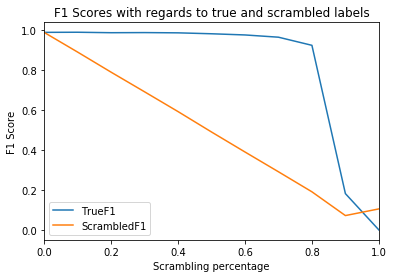
Comparing the F1 scores with regards to the true and the scrambled labels reveals a remarkable characteristic: the model is capable of learning the true relationship between input data and target variables even when up to
ax = results.plot(title="F1 Scores with regards to true and scrambled labels")
ax.set_xlabel("Scrambling percentage");
ax.set_ylabel("F1 Score");A neural network is clearly capable of learning the correct relationship between input data and target variables, even when training labels have been partially falsified. Astonishingly, the true performance doesn't gradually decrease but abruptly fails. In this case, the model performed near-perfectly up to a scrambling percentage of approximately
It needs to be said that the MNIST handwritten digits dataset is remarkably simple, which explains the high threshold. More complex datasets will have a lower threshold but should nevertheless elicit the same behaviour in models trained on noisy data.

