OPERA

Setting: when is the package opera useful?
Installation
Example: predict the weekly electricity consumption.

opera is a python package that provides several algorithms to perform robust online prediction of time series with the help of expert advice. In this vignette, we provide an example of how to use the package.

Also available on R : let's go !

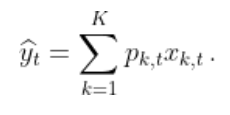
Setting: when is the package `opera` useful?

Consider a sequence of real bounded observations y₁, …, y_n to be predicted step by step. Suppose that you have at your disposal a finite set of methods k = 1, …, K (henceforth referred to as experts) that provide you before each time step t = 1, …, n predictions x_k, t of the next observation y_t. You can form your prediction ŷ_t by using only the knowledge of the past observations y₁, …, y_t − 1 and past and current expert forecasts x_k, 1, …, x_k, t for k = 1, …, K. The package opera implements several algorithms of the online learning literature that form predictions ŷ_t by combining the expert forecasts according to their past performance. That is,

These algorithms come with finite time worst-case guarantees. The monograph of Cesa-Bianchi and Lugisi (2006) gives a complete introduction to the setting of prediction of arbitrary sequences with the help of expert advice.

What are the most important functions?

The package opera provides the mixture class to build the algorithm object. The class contain three important functions:

update to update the class with new experts and new y.
predict to make a prediction by using the algorithm.
plot_mixture to provide different diagnostic plots for an aggregation procedure.

Installation

opera is not available on pypi, in order to install it you need to run the following command in the root directory:

pip install .

Example: predict the weekly electricity consumption.

Here, we provide a concrete example on how to use the package. The data are provided in the folder data.

The dataset contains three experts in experts.csv and the corresponding targets in targets.csv.

More information about the dataset can be found here.

Load the datasets

import pandas as pd
targets = pd.read_csv("data/targets.csv")["x"]
experts = pd.read_csv("data/experts.csv")

Aggregate the experts online using one of the possible aggregation procedures

The first step consists in initializing the algorithm by defining the type of algorithm (BOA, MLpol,…), the experts and targets, the possible parameters, and the evaluation criterion. Bellow, we define the ML-Poly algorithm, evaluated by the square loss.

from opera import Mixture
MLPOL1 = Mixture(
    y=targets.iloc[0:100],
    experts=experts.iloc[0:100],
    model="MLpol",
    loss_type="mse",
    loss_gradient=False,
)

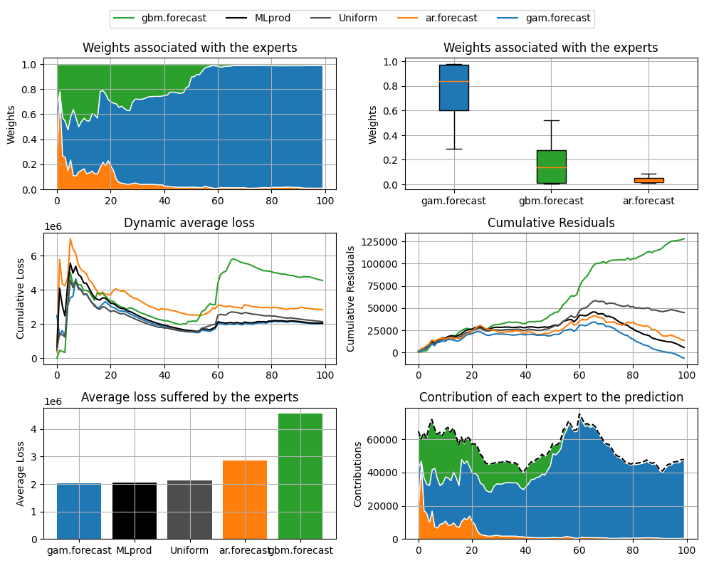
The results can be displayed with method plot_mixture.

MLPOL1.plot_mixture()

The same results can also be obtained by initializing the mixture with some data and updating it later:

MLPOL2 = Mixture(
    y=targets.iloc[0:50],
    experts=experts.iloc[0:50],
    awake=awake[0:50],
    model=model,
    loss_type="mse",
    loss_gradient=False,
)

MLPOL2.update(
    new_experts=experts.iloc[50:100], new_y=targets.iloc[50:100], awake=awake[50:100]
)

About the predictions

The vector of predictions formed by the mixture can be obtained through the output prediction.

predictions = MLPOL1.predictions

Note that these predictions were obtained sequentially by the algorithm by updating the model coefficients after each data. It is worth to emphasize that each observation is used to get the prediction of the next observations but not itself (nor past observations).

In real-world situations, predictions should be produced without having access to the observed outputs. There are two solutions to get them with opera.

Using the predict method : the model coefficients are not updated during the prediction.

newexperts = experts.iloc[-10:] # last ten observations of the dataset 
pred = MLPOL1.predict(new_experts = newexperts)
print(pred)

# array([[53308.36828688],
#        [57099.33148933],
#        [56767.62097983],
#        [55611.67204501],
#        [57256.02185278],
#        [61655.81982573],
#        [65022.29207561],
#        [72666.72935961],
#        [68171.64429055],
#        [60642.5452753 ]])

The same result can be easily obtained by using the last model coefficients to perform the weighted sum of the expert advice.

import numpy as np
pred = np.sum(newexperts * MLPOL1.w, axis=1)
print(pred)
# array([[53308.36828688],
#        [57099.33148933],
#        [56767.62097983],
#        [55611.67204501],
#        [57256.02185278],
#        [61655.81982573],
#        [65022.29207561],
#        [72666.72935961],
#        [68171.64429055],
#        [60642.5452753 ]])

Dralliag/opera-python