EMODnet-Biology-Benthos-Interpolated-Maps

DIVA (Data Interpolating Variational Analysis) and DIVAnd (DIVA in n dimensions) are software tools designed to generate gridded maps of continuous variables such as sea water temperature, salinity or oxygen concentration. The main advantages over other interpolation or analysis method are:

coastlines and physical boundaries are taken into account by the method.
large datasets (million of data points) can be ingested and processed by the tool.

DIVAnd is a multi-dimensional generalization (Barth et al., 2014), written in the Julia language, with a new mathematical formulation with respect to the previous DIVA code.

This directory provides the codes and tools to

process the presence/absence data relative to different benthos species, and
generate the gridded and error fields using DIVAnd.

DIVAnd for presence/absence data

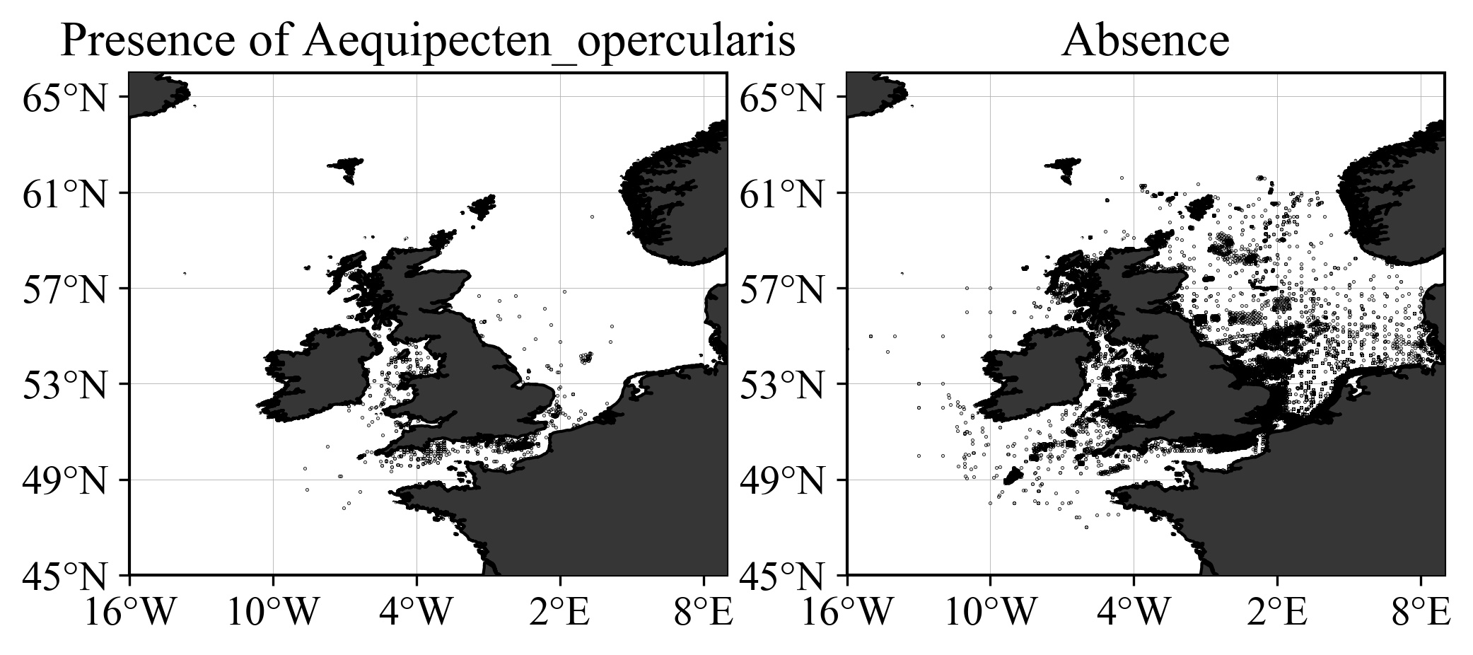
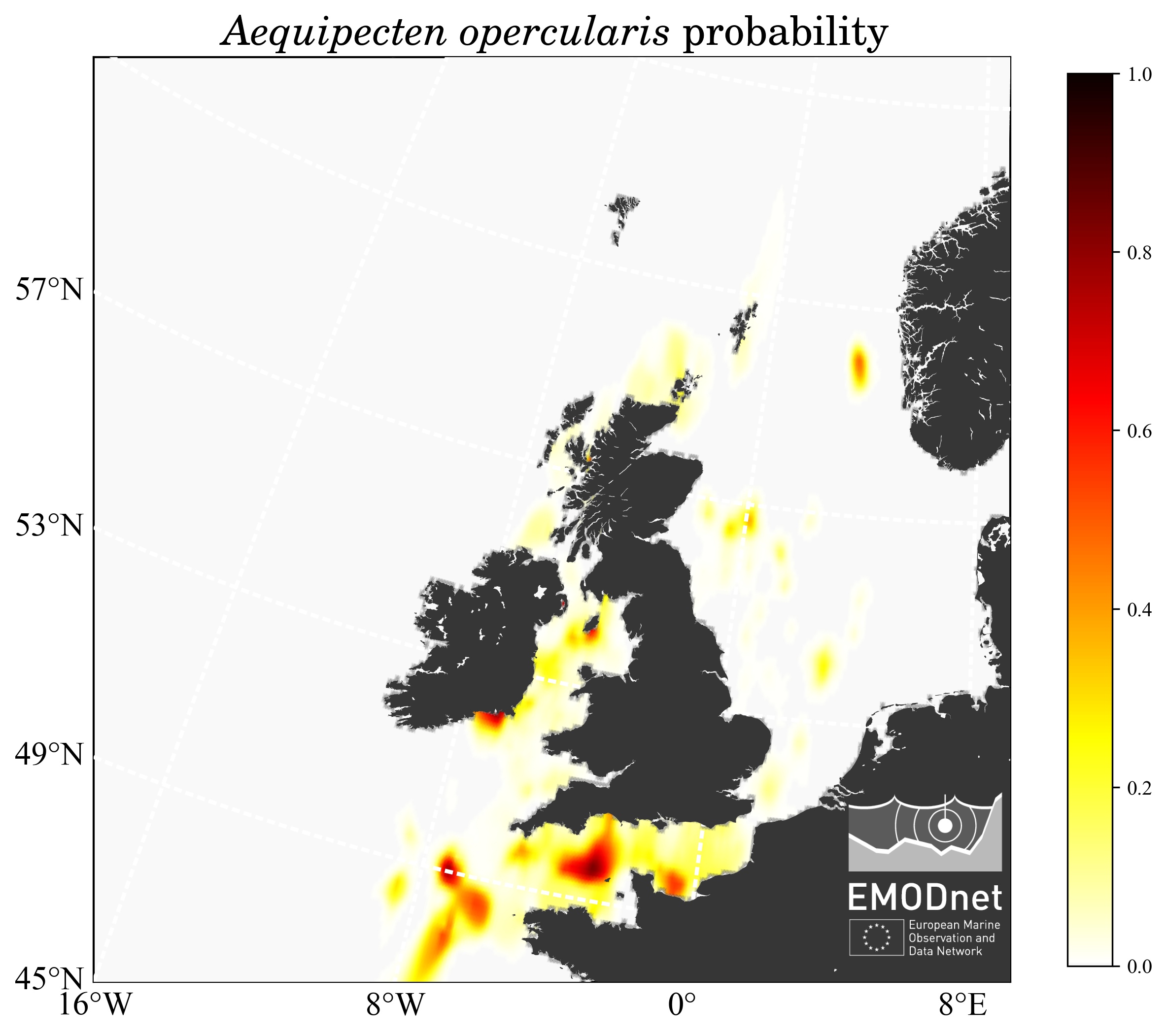
The dataset to be processed contained only a binary information: presence or absence, and the objective is to derive a map showing the probability to encounter a given species, as illustrated below for Aequipecten opercularis.

Directory structure

EMODnet-Biology-Benthos-Interpolated-Maps/
├── analysis
├── data/
├── docs/
├── product/
│   ├── figures/
│   └── netCDF/
└── scripts/

analysis - Jupyter notebooks used to perform the data analysis, create the figures and the netCDF files.
data - input data files.
docs - Rendered reports
product - Output product files: netCDF containing the gridded, probability fields and the corresponding figures in PNG or JPG format.
scripts - Reusable code: functions employed in the Jupyter notebooks.

Data series

The input data was provided by Herman et al (2020). The main data file is spe.csv, it contains all sampling events as rows, and the most frequent species (occurrence >200) as columns. The first columns specify sampling event and location. All columns are coded as ‘pa’ (for presence/absence) followed by the AphiaID of the species. In the separate file specieslist.csv you find the names of the species corresponding to their AphiaID. You also find the total number of events where the species has been found.

A species can have value 1 (present), 0 (looked for but absent) and NA (not looked for). The NA values must be disregarded when making maps. They do not contain information about either presence or absence. There are NAs in the file because some datasets only look for a subset of species.

The information about the occurrence of a species is obtained with the function read_coords_species defined in the script BenthosInterp.jl. The species are selected by using the AphiaID.

Data product

This directory contains the notebooks for the preparation and analysis of the data, as well as the generation of the figures.

Method

For a given species, two heatmaps are computed: one of the presence, the other for the absences. Then the probability (between 0 and 1) is computed using the following formula:

d = npre * dens_pre / (npre * dens_pre + nabs * dens_abs)

where

npre is the total number of absence data points;
nabs is the total number of absence data point;
dens_pre is the heatmap obtained with the presence data only;
dens_abs is the heatmap obtained with the absence data only.

If we have only presence data, the 2nd term of the denominator is zero and the probability reduces to the presence heatmap. The absence data decrease the ratio and hence the probability.

Jupyter notebooks

interp_presence_absence_benthos:

prepare the domain and the bathymetry,
read the coordinates of presence and absence for each species,
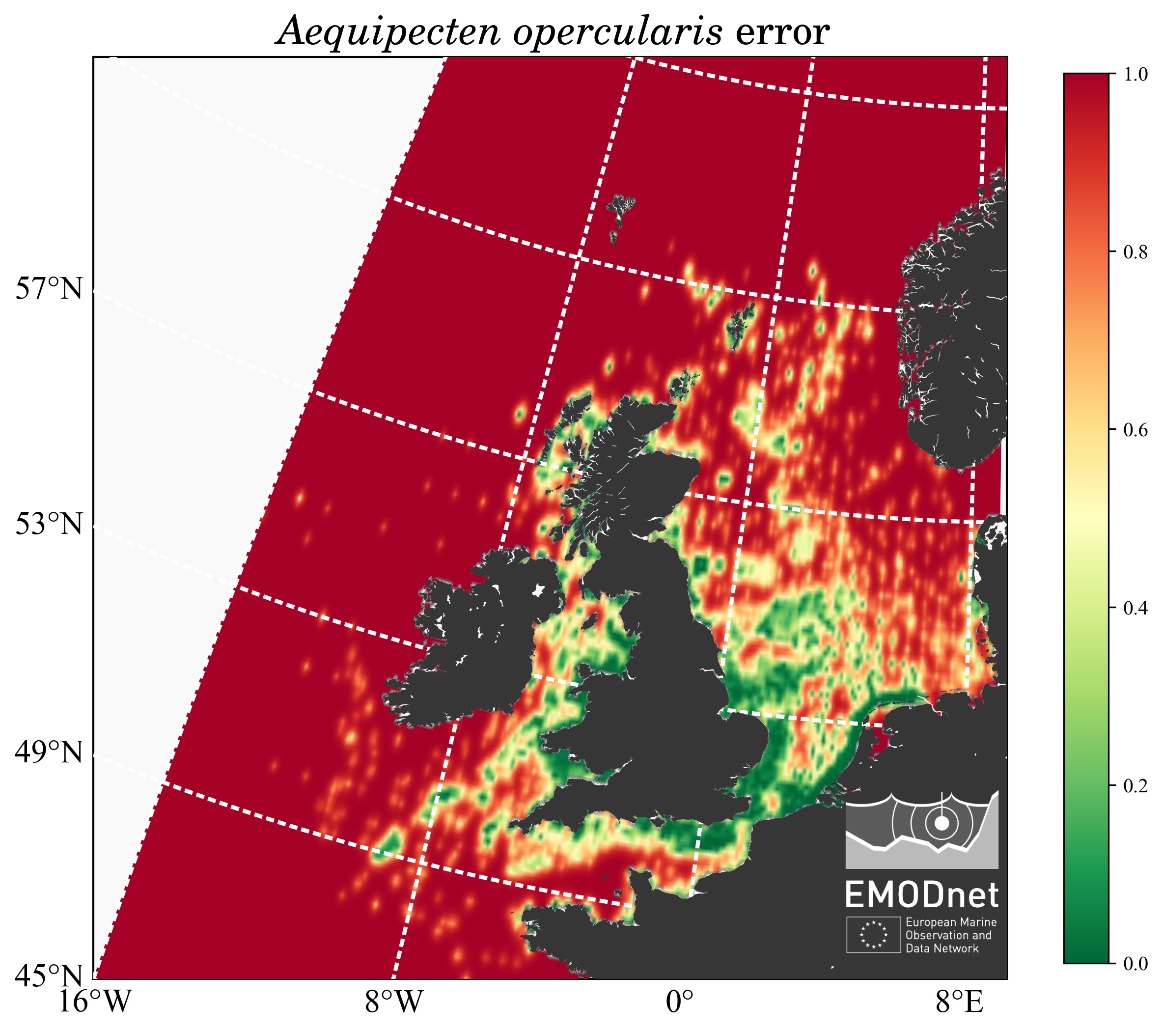
compute the probability map and the associated error field and
write the results in a netCDF file (one per species and one global for all the species), in the directory product/netCDF

plot_results_map.ipynb: notebook in Python to create the figures using the ETRS89 Lambert Azimuthal Equal Area coordinate reference system of 2001 (EPGS 3035).
The figures are stored in product/figures and consist of

The interpolated probability map
The relative error field
The interpolated probability masked by the error field: for some species the computed probability displays high and non-realistic values, due to the ratio of very small (but different) values in regions without observations.

Installation

You need Julia 1.5 (or later) available from https://julialang.org/downloads/. The following Julia packages required to run this code can be installed with:

using Pkg
Pkg.add("DIVAnd")
Pkg.add("DelimitedFiles")
Pkg.add("Dates")
Pkg.add("NCDatasets")
Pkg.add("GridInterpolations")
Pkg.add("Interpolations")
Pkg.add("Missings")

if plots are to be created with Julia, those packages are also required:

Pkg.add("PyCall")
Pkg.add("PyPlot")
Pkg.add("Proj4")

Products

Two types of analysis are performed:

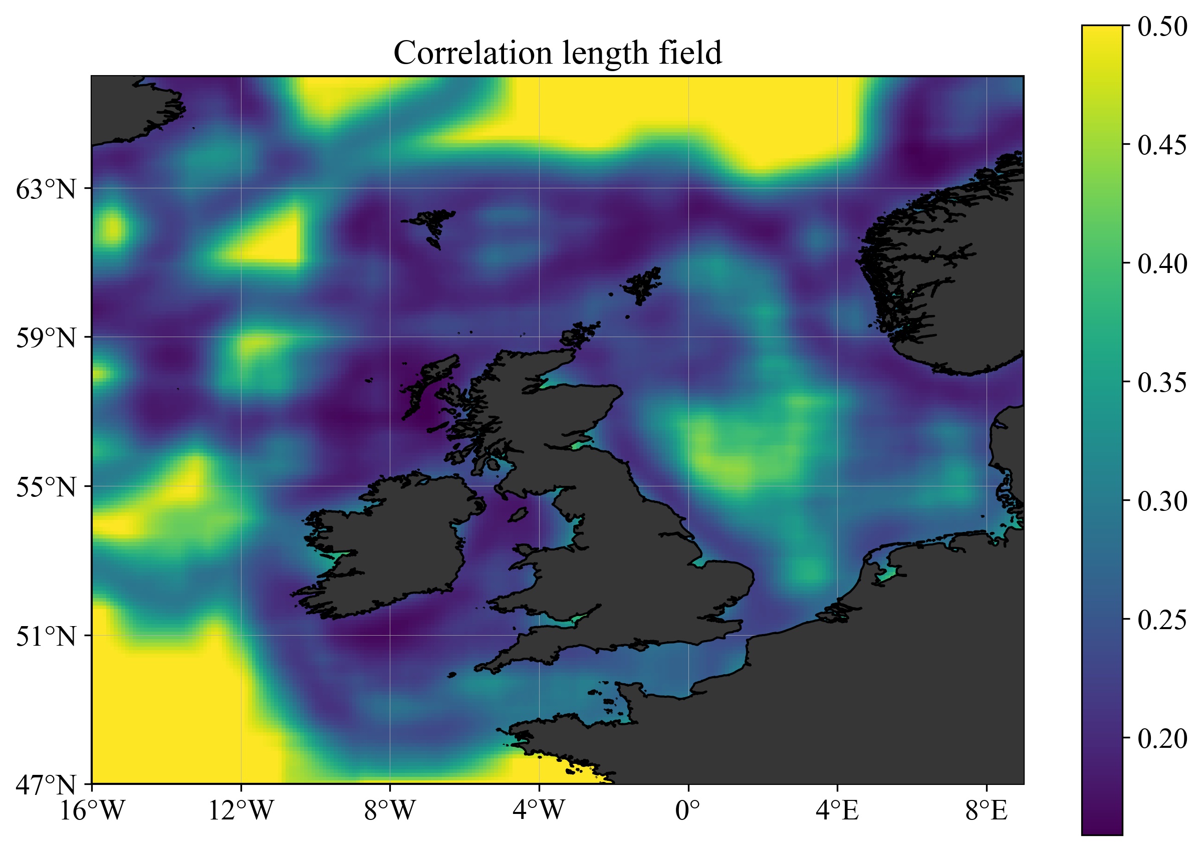
Using a uniform correlation length all over the domain (0.1°) (directory 1-UniformL)
Using a spatially variable correlation length (see figure below), derives from the substrates (directory 2-VariableL).

For both analysis, 2 types of products are created (described in the next section):

Figures (jpg format).
NetCDF files.

More information

References

Barth, A., Beckers, J.-M., Troupin, C., Alvera-Azcárate, A., and Vandenbulcke, L.(2014): divand-1.0: n-dimensional variational data analysis for ocean observations, Geosci. Model Dev., 7, 225–241, https://doi.org/10.5194/gmd-7-225-2014.

Herman, P.M.J., Stolte, W., van der Heijden, L. 2020. Summary presence/absence maps of macro-endobenthos in the greater North Sea, based on nearly 100,000 samples from 65 assembled monitoring data sets. Integrated data products created under the European Marine Observation Data Network (EMODnet) Biology project (EASME/EMFF/2017/1.3.1.2/02/SI2.789013), funded by the European Union under Regulation (EU) No 508/2014 of the European Parliament and of the Council of 15 May 2014 on the European Maritime and Fisheries Fund. Available at: https://www.emodnet-biology.eu/data-catalog?module=dataset&dasid=6617

Code and methodology

The code, written in Julia, is distributed through GitHub: https://github.com/EMODnet/EMODnet-Biology-Benthos-Interpolated-Maps

Citation and download link

Please cite this product as: A. Barth, P. Hermann and C. Troupin (2020). Probability maps for different benthos species in the North Sea. Integrated data products created under the European Marine Observation Data Network (EMODnet) Biology project (EASME/EMFF/2017/1.3.1.2/02/SI2.789013), funded by the European Union under Regulation (EU) No 508/2014 of the European Parliament and of the Council of 15 May 2014 on the European Maritime and Fisheries Fund.

The code is free software; you can redistribute it and/or modify it under the terms of the GNU General Public License as published by the Free Software Foundation; either version 2 of the License, or (at your option) any later version.

The product is available to download at:

Authors

A. Barth, P. Hermann and C. Troupin

Acknowledgement

Computational resources have been provided by the Consortium des Équipements de Calcul Intensif (CÉCI), funded by the Fonds de la Recherche Scientifique de Belgique (F.R.S.-FNRS) under Grant No. 2.5020.11 and by the Walloon Region"