The mixed models special agent (mimosa) is a shiny (Chang, Cheng,
Allaire, Xie, & McPherson, 2019) app for 2-level mixed models. Mixed
models are rapidly becoming the gold standard of statistical analysis
techniques in the behavioral sciences. Yet there is only a small number
of user-friendly programs for conducting mixed model analyses. The most
common tools often lack a graphical user interface, are proprietary, and
involve a tedious process of getting data in and publication-ready
tables out. An exception is the shiny app mimosa which offers an
alternative that is free, open source, intuitive, and runs in a browser,
making it easily accessible (see https://www.mimosa.icu).
The software is targeted at behavioral scientists who frequently use
2-level mixed models and want a solution that is tailored for this
particular use case. For instance, researchers studying groups
(e.g. students clustered in schools, individuals clustered in work
groups) and researchers employing within-subjects designs almost
exclusively analyze their data with 2-level mixed models. Unlike other
software, mimosa was designed for this use case. It helps the analyst
by automatically detecting potential grouping variables and categorizing
these variables in level 1 and level 2. Furthermore, mimosa is
researcher-oriented because it produces a single summary table via
sjPlot (Lüdecke, 2018) that can be published in a scientific journal
without any modifications.
These benefits come at the cost of the limitation to 2-level models. If
you need to model more complex cases, mimosa might not be suited for
you and you should check out the more comprehensive software GAMLj
(Gallucci, 2020).
No need to install mimosa, just go to www.mimosa.icu and use it there. An example data file is loaded when you go to www.mimosa.icu/example.
If you really want to use it locally, install from github (you need the package devtools for this):
devtools::install_github("johannes-titz/mimosa")And now run the app:
mimosa::run_app()Yes, it is that easy—at least under GNU/Linux!
If you have any problems installing mimosa, check that your R version is up to date (currently 3.6.2). If you are using Windows, enable TLS 1.2 in the Internet Options Advanced tab (see r-lib/remotes#130 (comment)). Under Windows, you will also need Rtools to build the package: https://cran.r-project.org/bin/windows/Rtools/.
If it still does not work drop me an e-mail at johannes at titz.science or at johannes.titz at gmail.com.
As an example data set we will use exam scores of 4,059 students from 65
schools in Inner London (Goldstein et al., 1993), which is available in
the R package mlmRev (Bates, Maechler, & Bolker, 2019). The variables
are described in the table below. Here, we will focus on the exam score
as the outcome variable and use LRT and school type as a predictor. The
standardized exam score is a total score of different subjects taken in
a public examination at age 16. LRT is the London Reading Test, taken at
the age of 11. Both variables are already
-standardized in the
data set. The other variables are described in more detail in Goldstein
et al. (1993) and Nuttall, Goldstein, Prosser, & Rasbash (1989).
| variable | description | data type | levels (if factor) |
|---|---|---|---|
| school | school ID | factor | 65 levels |
| normexam | standardized exam score | numeric | |
| schgend | school gender | factor | mixed, boys, girls |
| schavg | school average of intake score | numeric | |
| vr | student level Verbal Reasoning (VR) score band at intake | factor | bottom 25%, mid 50%, top 25% |
| intake | band of student’s intake score | factor | bottom 25%, mid 50%, top 25% |
| standLRT | standardized listening and reading test score | numeric | |
| sex | sex of the student | factor | F, M |
| type | school type | factor | Mxd, Sngl |
| student | student ID (within school) | factor | 650 levels |
Description of example
data. Note. This data is available in the R package mlmRev (Bates et
al., 2019) and is from the study by Goldstein et al. (1993).
If you want to follow the example you can now go to www.mimosa.icu/example, which will automatically load the school data set. A big improvement over existing software is that mimosa detects the grouping variable and the hierarchical levels in the data automatically when the data is loaded:
In the school data set, school is indeed the grouping variable. The automatic selection process works by analyzing the structure of the data. For every potential grouping variable, mimosa checks how many level-2 variables would be created and how many different levels exist on average. Based on this, many variables can be excluded as grouping variables and the remaining ones can be ordered by the likelihood of being the correct grouping variable. This heuristic works surprisingly well. It has been tested with a dozen of real data files that have a 2-level structure and mimosa was always able to guess the correct grouping variable. Even if the heuristic should fail, one can select the correct grouping variable manually.
If the grouping variable is known, the procedure to categorize variables in level 1 and level 2 is as follows: Take a variable and group it by the grouping variable. Then, determine the number of unique levels of the variable (for each group). If the variable is on the second level, the number of unique levels should be one for each group. As an example, consider the school data set. It has 65 schools and a variable on the second level is schgend, the school gender (mixed, boys, girls). For every school, the school gender is constant, so this is a level-2 variable.
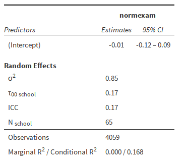
Model specification is quite self-explanatory: First one determines the dependent variable, for which the exam score (normexam) appears most interesting in the school data set (see image above). The output for this null model is directly created with the most useful statistics:
The null model produces an intercept of close to 0, which makes sense
since the data is standardized. The output table is created with
sjPlot (Lüdecke, 2018). It is concise, nicely formatted and can be
either downloaded as an HTML file or directly copy-pasted to the
application of choice (e.g. a word processor). Additional statistics
(standard error, AIC, deviance, Log-Likelihood, standardized
coefficients, test statistic,
-value), can be selected
in the Table Options dialog (not shown here).
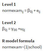
The model description is shown mathematically and in R syntax of the
lme4 package:
In the next step one can select the independent variables on level 1,
after which one can further specify if these variables should be modeled
as random or fixed effects. For the example data set, one can add
standLRT (a standardized listening and reading test score). The output
table as well as the model description adapts each time a change is
made. Note that, to avoid redundancy, this updated table is not shown
here, but you can check the results on your own at
www.mimosa.icu/example. The effect for
standLRT is .56. One can add a random component to the effect, which
will result in an estimate for the variance in the population of the
standLRT effect (not shown here). It is only 0.01,
but the square root
is usually more interesting, giving the estimated
population standard deviation for the estimated population effect of
.56.
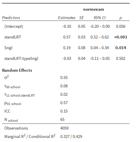
In the following step, one can add a variable on level 2, for instance type. The resulting model shows that, compared to mixed schools, single schools perform somewhat better (not displayed here). If at least one level-1 variable varies and a level-2 variable is selected, cross-level interactions can also be specified. If the level-1 variable does not vary, this option is not available because the idea of an interaction is that one can predict the size of an effect on level 1 by using a level-2 variable. In the exemplary analysis, only one interaction is available, between standLRT and type. By selecting it we arrive at the final model:
The effect of the interaction is about -0.03, meaning that the relationship between standLRT and normexam is a bit lower for single gender schools than for mixed gender schools. But the effect is not reliable since the confidence intervals are quite wide.
The general conclusion for the data set might be that a reading test at age 11 can predict the final exam grade at age 16 relatively well. Furthermore, single gender schools perform somewhat better than mixed gender schools. Overall, the model explains about 43% of the total variance, which is quite good for social science.
If you find any bugs, please use the issue tracker at:
https://github.com/johannes-titz/mimosa/issues
If you need answers on how to use the package, drop me an e-mail at johannes at titz.science or johannes.titz at gmail.com
Comments and feedback of any kind are very welcome! I will thoroughly consider every suggestion on how to improve the code, the documentation, and the presented examples. Even minor things, such as suggestions for better wording or improving grammar in any part of the package, are more than welcome.
If you want to make a pull request, please check that you can still build the package without any errors, warnings, or notes. Overall, simply stick to the R packages book: https://r-pkgs.org/ and follow the code style described here: http://r-pkgs.had.co.nz/r.html#style
I want to sincerely thank Maria Reichert for writing a first scaffold
for mimosa (see the initial commit). Further, I want to thank Markus
Burkhardt, Karin Matko, Thomas Schäfer, Peter Sedlmeier, and Isabell
Winkler for testing mimosa and giving helpful comments on the
documentation.
Bates, D., Maechler, M., & Bolker, B. (2019). mlmRev: Examples from multilevel modelling software review. Retrieved from https://CRAN.R-project.org/package=mlmRev
Chang, W., Cheng, J., Allaire, J. J., Xie, Y., & McPherson, J. (2019). Shiny: Web application framework for R. Retrieved from https://CRAN.R-project.org/package=shiny
Gallucci, M. (2020). GAMLj suite for jamovi. Retrieved from https://github.com/gamlj/gamlj
Goldstein, H., Rasbash, J., Yang, M., Woodhouse, G., Pan, H., Nuttall, D., & Thomas, S. (1993). A multilevel analysis of school examination results. Oxford Review of Education, 19, 425–433. https://doi.org/10.1080/0305498930190401
Lüdecke, D. (2018). sjPlot: Data visualization for statistics in social science. https://doi.org/10.5281/zenodo.1308157
Nuttall, D. L., Goldstein, H., Prosser, R., & Rasbash, J. (1989). Differential school effectiveness. International Journal of Educational Research, 13, 769–776. https://doi.org/10.1016/0883-0355(89)90027-X


